Lighting
Overview
The following sections of documentation attempt to describe the theory and
implementation of lighting in the
io7m-r1 package. All lighting
in the package is dynamic - there is no support
for precomputed lighting and all contributions from lights are recalculated every
time a scene is rendered. Lighting is configured by adding instances of
KLightType
to a scene.
Diffuse/Specular Terms
The light applied to a surface by a given light is divided
into diffuse and
specular terms
[31]. The actual light applied to a surface is dependent upon
the properties of the surface. Conceptually, the diffuse and specular
terms are multiplied by the final color of the surface and summed. In
practice, the materials applied to surfaces have control over how
light is actually applied to the surface. For example, materials may
include a
specular map
which is used to manipulate the specular term as it is applied to the surface.
Additionally, if a light supports attenuation,
then the diffuse and specular terms are scaled by the attenuation factor
prior to being applied.
The diffuse term is modelled by
Lambertian reflectance.
Specifically, the amount of diffuse light reflected from a surface
is given by diffuse
[LightDiffuse.hs]:
module LightDiffuse where

import qualified Color3
import qualified Direction
import qualified Normal
import qualified Spaces
import qualified Vector3f

diffuse ::  Direction.T Spaces.Eye -> Normal.T -> Color3.T -> Float -> Vector3f.T
diffuse stl n light_color light_intensity =
  let
    factor       = max 0.0 (Vector3f.dot3 stl n)
    light_scaled = Vector3f.scale light_color light_intensity
  in
    Vector3f.scale light_scaled factor
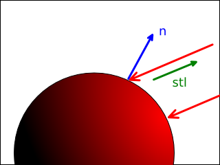
Where stl is a unit length direction vector
from the surface to the light source, n is the surface
normal vector, light_color is the
light color, and light_intensity
is the light intensity. Informally, the algorithm determines how much diffuse light
should be reflected from a surface based on how directly that surface
points towards the light. When stl == n,
Vector3f.dot3 stl n == 1.0, and
therefore the light is reflected exactly as received. When
stl is perpendicular to
n (such that
Vector3f.dot3 stl n == 0.0), no
light is reflected at all. If the two directions are greater than
90° perpendicular, the dot product
is negative, but the algorithm clamps negative values to
0.0 so the effect is the same.
The specular term is modelled by
Phong reflection
[32].
Specifically, the amount of specular light reflected from a surface is given by
specular
[LightSpecular.hs]:
module LightSpecular where

import qualified Color3
import qualified Direction
import qualified Normal
import qualified Reflection
import qualified Spaces
import qualified Specular
import qualified Vector3f

specular :: Direction.T Spaces.Eye -> Direction.T Spaces.Eye -> Normal.T -> Color3.T -> Float -> Specular.T -> Vector3f.T
specular stl view n light_color light_intensity (Specular.S surface_spec surface_exponent) =
  let
    reflection   = Reflection.reflection view n
    factor       = (max 0.0 (Vector3f.dot3 reflection stl)) ** surface_exponent
    light_raw    = Vector3f.scale light_color light_intensity
    light_scaled = Vector3f.scale light_raw factor
  in
    Vector3f.mult3 light_scaled surface_spec
Where stl is a unit length direction vector
from the surface to the light source,
view is a unit length
direction vector from the observer to the surface,
n is the surface
normal vector, light_color is the
light color, light_intensity
is the light intensity, surface_exponent is the
specular exponent defined by the surface,
and surface_spec is the surface
specularity factor.
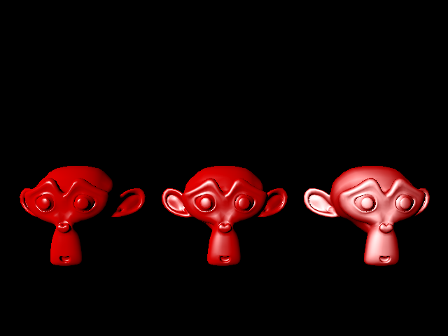
The specular exponent is a value, ordinarily in the range
[0, 255], that
controls how sharp the specular highlights
appear on the surface. The exponent is a property of the surface, as opposed
to being a property of the light. Low specular exponents result in soft and widely
dispersed specular highlights (giving the appearance of a rough surface), while
high specular exponents result in hard and focused highlights (giving the appearance of a polished
surface). As an example, three models lit with
progressively lower specular exponents from left to right (128,
32, and 8,
respectively):
Diffuse-Only Lights
Attenuation
Attenuation is the property of the influence
of a given light on a surface in inverse proportion to the distance from the
light to the surface. In other words, for lights that support attenuation,
the further a surface is from a light source, the less that surface will
appear to be lit by the light. For light types that support attenuation,
an attenuation factor is calculated based
on a given inverse_maximum_range
(where the maximum_range is a
light-type specific positive value that represents the maximum possible
range of influence for the light), a configurable
inverse falloff value, and the current
distance between the surface being
lit and the light source. The attenuation factor is a value in the range
[0.0, 1.0], with
1.0 meaning "no attenuation" and
0.0 meaning "maximum attenuation".
The resulting attenuation factor is multiplied by the raw unattenuated
light values produced for the light in order to produce the illusion of
distance attenuation. Specifically:
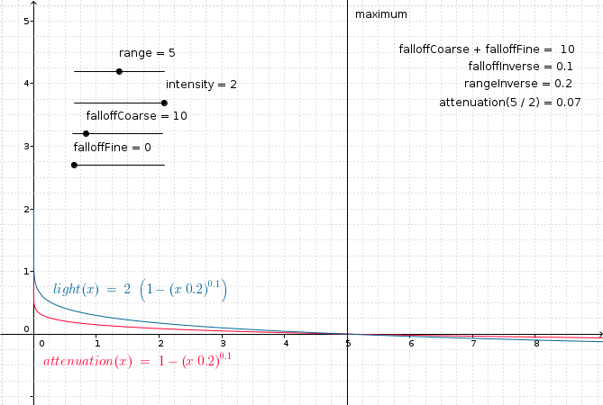
module Attenuation where

attenuation_from_inverses :: Float -> Float -> Float -> Float
attenuation_from_inverses inverse_maximum_range inverse_falloff distance =
  max 0.0 (1.0 - (distance * inverse_maximum_range) ** inverse_falloff)

attenuation :: Float -> Float -> Float -> Float
attenuation maximum_range falloff distance =
  attenuation_from_inverses (1.0 / maximum_range) (1.0 / falloff) distance
Given the above definitions, a number of observations can be made.
If maximum_range == 0, then the
inverse range is undefined, and therefore the results of lighting are
undefined. The io7m-r1 package
handles this case by raising an exception when the light is created.
If falloff == 0, then the
inverse falloff is undefined, and therefore the results of lighting are
undefined. The io7m-r1 package
handles this case by raising an exception when the light is created.
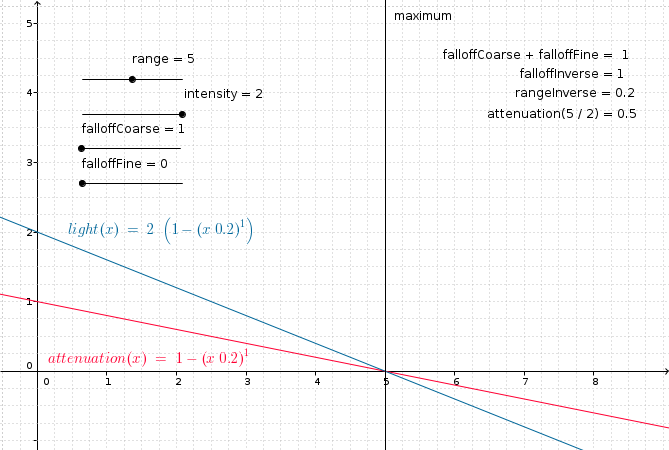
As falloff decreases towards
0.0, then the attenuation curve
remains at 1.0 for increasingly
higher distance values before falling sharply to
0.0:
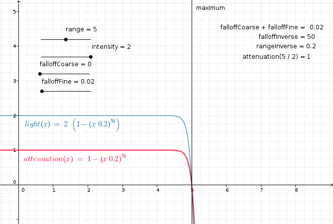
As falloff increases away from
0.0, then the attenuation curve
decreases more for lower distance values:
[31]
The io7m-r1 package
does not use ambient terms.
[32]
Note: Specifically Phong reflection
and not the more commonly used
Blinn-Phong reflection.
[33]
The attenuation function development is available for experimentation
in the included GeoGebra
file [attenuation.ggb].