com.io7m.r2 0.3.0-SNAPSHOT Documentation
- 1. Package Information
- 2. Design And Implementation
- 2.1. Conventions
- 2.2. Concepts
- 2.3. Coordinate Systems
- 2.4. Meshes
- 2.5. Transforms
- 2.6. Instances
- 2.7. Render Targets
- 2.8. Shaders
- 2.9. Shaders: Instance
- 2.10. Shaders: Light
- 2.11. Stencils
- 2.12. Lighting
- 2.13. Lighting: Directional
- 2.14. Lighting: Spherical
- 2.15. Lighting: Projective
- 2.16. Shadows
- 2.17. Shadows: Variance Mapping
- 2.18. Deferred Rendering
- 2.19. Deferred Rendering: Geometry
- 2.20. Deferred Rendering: Lighting
- 2.21. Deferred Rendering: Position Reconstruction
- 2.22. Forward rendering (Translucency)
- 2.23. Normal Mapping
- 2.24. Logarithmic Depth
- 2.25. Environment Mapping
- 2.26. Stippling
- 2.27. Generic Refraction
- 2.28. Filter: Fog
- 2.29. Filter: Screen Space Ambient Occlusion
- 2.30. Filter: Emission
- 2.31. Filter: FXAA
- 3. API Documentation
Package Information
Orientation
Features
- A deferred rendering core for opaque objects.
- A forward renderer, supporting a subset of the features of the deferred renderer, for rendering translucent objects.
- A full dynamic lighting system, including variance shadow mapping. The use of deferred rendering allows for potentially hundreds of dynamic lights per scene.
- Ready-to-use shaders providing surfaces with a wide variety of effects such as normal mapping, environment-mapped reflections, generic refraction, surface emission, mapped specular highlights, etc.
- A variety of postprocessing effects such as box blurring, screen-space ambient occlusion (SSAO), fast approximate antialiasing (FXAA), color correction, bloom, etc. Effects can be applied in any order.
- Explicit control over all resource loading and caching. For all transient resources, the programmer is required to provide the renderer with explicit pools, and the pools themselves are responsible for allocating and loading resources.
- Extensive use of static types. As with all io7m packages, there is extreme emphasis on using the type system to make it difficult to use the APIs incorrectly.
- Portability. The renderer will run on any system supporting OpenGL 3.3 and Java 8.
- A scene graph. The renderer expects the programmer to provide a set of instances (with associated shaders) and lights once per frame, and the renderer will obediently draw exactly those instances. This frees the programmer from having to interact with a clumsy and type-unsafe object-oriented scene graph as with other 3D engines, and from having to try to crowbar their own program's data structures into an existing graph system.
- Spatial partitioning. The renderer knows nothing of the world the programmer is trying to render. The programmer is expected to have done the work of deciding which instances and lights contribute to the current image, and to provide only those lights and instances for the current frame. This means that the programmer is free to use any spatial partitioning system desired.
- Input handling. The renderer knows nothing about keyboards, mice, joysticks. The programmer passes an immutable snapshot of a scene to the renderer, and the renderer returns an image. This means that the programmer is free to use any input system desired without having to painfully integrate their own code with an existing input system as with other 3D engines.
- Audio. The renderer makes images, not sounds. This allows programmers to use any audio system they want in their programs.
- Skeletal animation. The input to the renderer is a set of triangle meshes in the form of vertex buffer objects. This means that the programmer is free to use any skeletal animation system desired, providing that the system is capable of producing vertex buffer objects of the correct type as a result.
- Model loading. The input to the renderer is a set of triangle meshes in the form of vertex buffer objects. This means that the programmer is free to use any model loading system desired, providing that the system is capable of producing vertex buffer objects of the correct type as a result.
- Future proofing. The average lifetime of a rendering system is about five years. Due to the extremely rapid pace of advancement in graphics hardware, the methods use to render graphics today will bear almost no relation to those used five years into the future. The r2 package is under no illusion that it will still be relevant in a decade's time. It is designed to get work done today, using exactly those techniques that are relevant today. It will not be indefinitely expanded and grown organically, as this would directly contradict the goal of having a minimalist and correct rendering system.
- OpenGL ES 2 support. The ES 2 standard was written as a reaction to the insane committee politics that plagued the OpenGL 2.* standards. It is crippled to the point that it essentially cannot support almost any of the rendering techniques present in the r2 package, and is becoming increasingly irrelevant as the much saner ES 3 is adopted by hardware vendors.
Installation
Source compilation
$ mvn -C clean install
Maven
Regular releases are made to the Central Repository, so it's possible to use the com.io7m.r2 package in your projects with the following Maven dependencies:
<dependency>
  <groupId>com.io7m.r2</groupId>
  <artifactId>io7m-r2-main</artifactId>
  <version>0.3.0-SNAPSHOT</version>
</dependency>
License
All files distributed with the com.io7m.r2 package are placed under the following license:
Copyright © 2016 <code@io7m.com> http://io7m.com

Permission to use, copy, modify, and/or distribute this software for any
purpose with or without fee is hereby granted, provided that the above
copyright notice and this permission notice appear in all copies.

THE SOFTWARE IS PROVIDED "AS IS" AND THE AUTHOR DISCLAIMS ALL WARRANTIES
WITH REGARD TO THIS SOFTWARE INCLUDING ALL IMPLIED WARRANTIES OF
MERCHANTABILITY AND FITNESS. IN NO EVENT SHALL THE AUTHOR BE LIABLE FOR
ANY SPECIAL, DIRECT, INDIRECT, OR CONSEQUENTIAL DAMAGES OR ANY DAMAGES
WHATSOEVER RESULTING FROM LOSS OF USE, DATA OR PROFITS, WHETHER IN AN
ACTION OF CONTRACT, NEGLIGENCE OR OTHER TORTIOUS ACTION, ARISING OUT OF
OR IN CONNECTION WITH THE USE OR PERFORMANCE OF THIS SOFTWARE.
Design And Implementation
- 2.1. Conventions
- 2.2. Concepts
- 2.3. Coordinate Systems
- 2.4. Meshes
- 2.5. Transforms
- 2.6. Instances
- 2.7. Render Targets
- 2.8. Shaders
- 2.9. Shaders: Instance
- 2.10. Shaders: Light
- 2.11. Stencils
- 2.12. Lighting
- 2.13. Lighting: Directional
- 2.14. Lighting: Spherical
- 2.15. Lighting: Projective
- 2.16. Shadows
- 2.17. Shadows: Variance Mapping
- 2.18. Deferred Rendering
- 2.19. Deferred Rendering: Geometry
- 2.20. Deferred Rendering: Lighting
- 2.21. Deferred Rendering: Position Reconstruction
- 2.22. Forward rendering (Translucency)
- 2.23. Normal Mapping
- 2.24. Logarithmic Depth
- 2.25. Environment Mapping
- 2.26. Stippling
- 2.27. Generic Refraction
- 2.28. Filter: Fog
- 2.29. Filter: Screen Space Ambient Occlusion
- 2.30. Filter: Emission
- 2.31. Filter: FXAA
Conventions
Overview
This section attempts to document the mathematical and typographical conventions used in the rest of the documentation.
Mathematics
Rather than rely on untyped and ambiguous mathematical notation, this documentation expresses all mathematics and type definitions in strict Haskell 2010 with no extensions. All Haskell sources are included along with the documentation and can therefore be executed from the command line GHCi tool in order to interactively check results and experiment with functions.
When used within prose, functions are usually referred to using fully qualified notation, such as (Vector3f.cross n t). This is the application of the cross function defined in the Vector3f module, to the arguments n and t.
Concepts
- 2.2.1. Overview
- 2.2.2. Renderer
- 2.2.3. Render Target
- 2.2.4. Geometry Buffer
- 2.2.5. Light Buffer
- 2.2.6. Mesh
- 2.2.7. Transform
- 2.2.8. Instance
- 2.2.9. Light
- 2.2.10. Light Clip Group
- 2.2.11. Light Group
- 2.2.12. Shader
- 2.2.13. Material
Overview
This section attempts to provide a rough overview of the concepts present in the r2 package. Specific implementation details, mathematics, and other technical information is given in later sections that focus on each concept in detail.
Renderer
A renderer is a function that takes an input of some type and produces an output to a render target.
The renderers expose an interface of stateless functions from inputs to outputs. That is, the renderers should be considered to simply take input and produce return images as output. In reality, because the Java language is not pure and because the code is required to perform I/O in order to speak to the GPU, the renderer functions are not really pure. Nevertheless, for the sake of ease of use, lack of surprising results, and correctness, the renderers at least attempt to adhere to the idea of pure functional rendering! This means that the renderers are very easy to integrate into any existing system: They are simply functions that are evaluated whenever the programmer wants an image. The renderers do not have their own main loop, they do not have any concept of time, do not remember any images that they have produced previously, do not maintain any state of their own, and simply write their results to a programmer-provided render target. Passing the same input to a renderer multiple times should result in the same image each time.
Render Target
A render target is a rectangular region of memory allocated on the GPU that can accept the results of a rendering operation. The programmer typically allocates one render target, passes it to a renderer along with a renderer-specific input value, and the renderer populates the given render target with the results. The programmer can then copy the contents of this render target to the screen for viewing, pass it on to a separate filter for extra visual effects, use it as a texture to be applied to objects in further rendered images, etc.
Geometry Buffer
A geometry buffer is a specific type of render target that contains the surface attributes of a set of rendered instances. It is a fundamental part of deferred rendering that allows lighting to be efficiently calculated in screen space, touching only those pixels that will actually contribute to the final rendered image.
Light Buffer
A light buffer is a specific type of render target that contains the summed light contributions for each pixel in the currently rendered scene.
Mesh
A mesh is a collection of vertices that define a polyhedral object, along with a list of indices that describe how to make triangles out of the given vertices.
Transform
A transform moves coordinates in one coordinate space to another. Typically, a transform is used to position and orient a mesh inside a visible set.
Instance
An instance is essentially an object or group of objects that can be rendered. Instances come in several forms: single, batched, and billboarded.
A batched instance consists of a reference to a mesh and an array of transforms. The results of rendering a batched instance are the same as if a single instance had been created and rendered for each transform in the array. The advantage of batched instances is efficiency: Batched instances are submitted to the GPU for rendering in a single draw call. Reducing the total number of draw calls per scene is an important optimization on modern graphics hardware, and batched instances provide a means to achieve this.
A billboarded instance is a further specialization of a batched instance intended for rendering large numbers of objects that always face towards the observer. Billboarding is a technique that is often used to render large numbers of distant objects in a scene: Rather than incur the overhead of rendering lots of barely-visible objects at full detail, the objects are replaced with billboarded sprites at a fraction of the cost. There is also a significant saving in the memory used to store transforms, because a billboarded sprite need only store a position and scale as opposed to a full transform matrix per rendered object.
Light
A light describes a light source within a scene. There are many different types of lights, each with different behaviours. Lights may or may not cast shadows, depending on their type. All lighting in the r2 package is completely dynamic; there is no support for static lighting in any form. Shadows are exclusively provided via shadow mapping, resulting in efficient per-pixel shadows.
Light Clip Group
A light clip group is a means of constraining the contributions of groups of lights to a provided volume.
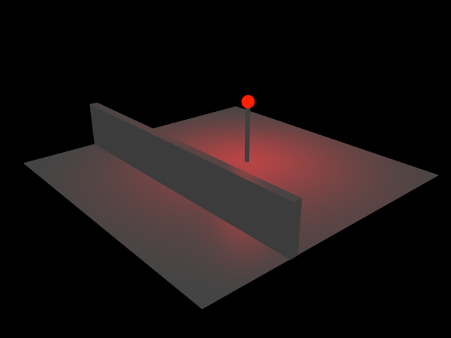
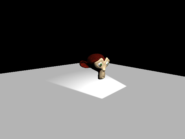
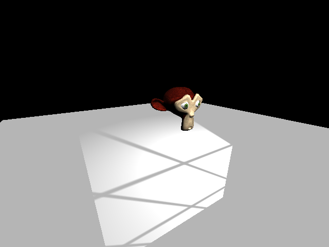
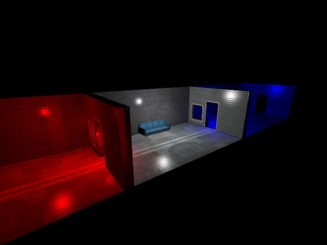
Because, like most renderers, the r2 package implements so-called local illumination, lights that do not have explicit shadow mapping enabled are able to bleed through solid objects:
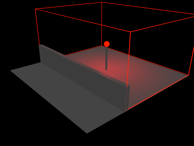
Enabling shadow mapping for every single light source would be prohibitively expensive [3], but for some scenes, acceptable results can be achieved by simply preventing the light source from affecting pixels outside of a given clip volume.
Light Group
A light group is similar to a light clip group in that is intended to constrain the contributions of a set of lights. A light group instead requires the cooperation of a renderer that can mark groups of instances using the stencil component of the current geometry buffer. At most 15 light groups can be present in a given scene, and for a given light group n, only instances in group n will be affected by lights in group n. By default, if a group is not otherwise specified, all lights and instances are rendered in group 1.
Shader
A shader is a small program that executes on the GPU and is used to produce images. The r2 package provides a wide array of general-purpose shaders, and the intention is that users of the package will not typically have to write their own [2].
The package roughly divides shaders into categories. Single instance shaders are typically used to calculate and render the surface attributes of single instances into a geometry buffer. Batched instance shaders do the same for batched instances. Light shaders render the contributions of light sources into a light buffer. There are many other types of shader in the r2 package but users are generally not exposed to them directly.
Coordinate Systems
- 2.3.1. Conventions
- 2.3.2. Object Space
- 2.3.3. World Space
- 2.3.4. Eye Space
- 2.3.5. Clip Space
- 2.3.6. Normalized-Device Space
- 2.3.7. Screen Space
Conventions
This section attempts to describe the mathematical conventions that the r2 package uses with respect to coordinate systems. The r2 package generally does not deviate from standard OpenGL conventions, and this section does not attempt to give a rigorous formal definition of these existing conventions. It does however attempt to establish the naming conventions that the package uses to refer to the standard coordinate spaces [10].
The r2 package uses the jtensors package for all mathematical operations on the CPU, and therefore shares its conventions with regards to coordinate system handedness. Important parts are repeated here, but the documentation for the jtensors package should be inspected for details.
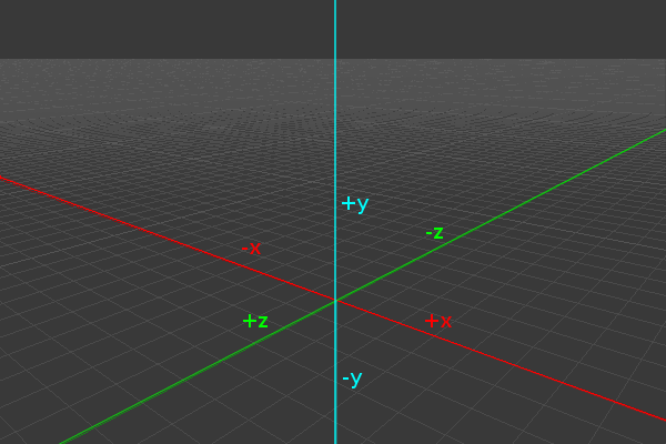
Any of the matrix functions that deal with rotations assume a right-handed coordinate system. This matches the system conventionally used by OpenGL (and most mathematics literature) . A right-handed coordinate system assumes that if the viewer is standing at the origin and looking towards negative infinity on the Z axis, then the X axis runs horizontally (left towards negative infinity and right towards positive infinity) , and the Y axis runs vertically (down towards negative infinity and up towards positive infinity). The following image demonstrates this axis configuration:
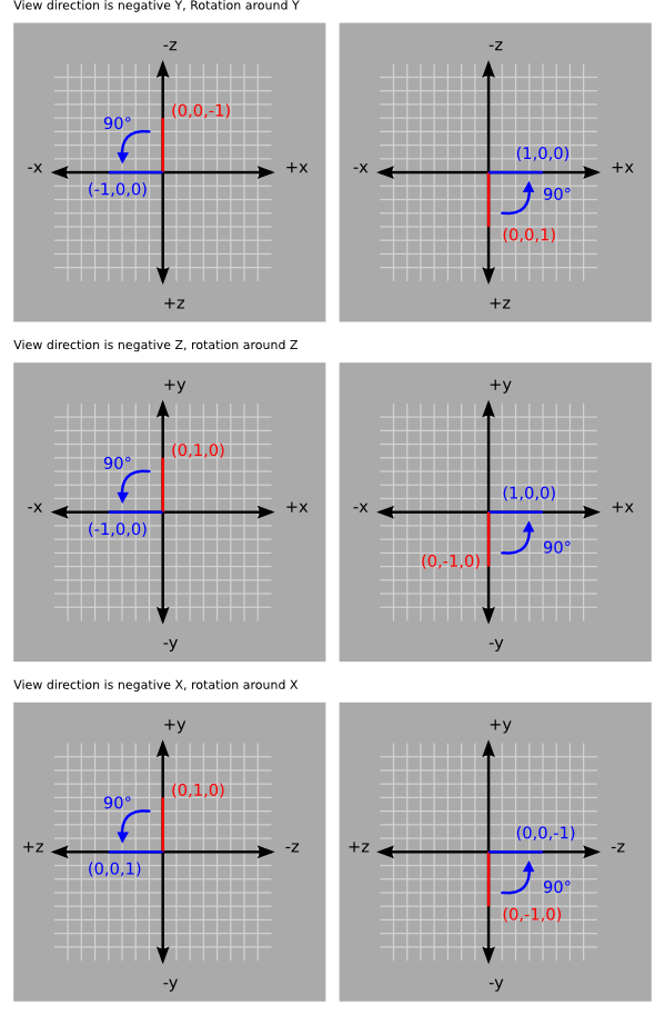
The jtensors package adheres to the convention that a positive rotation around an axis represents a counter-clockwise rotation when viewing the system along the negative direction of the axis in question.
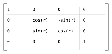
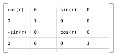
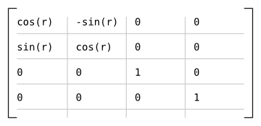
The package uses the following matrices to define rotations around each axis:
Which results in the following matrix for rotating r radians around the axis given by (x, y, z), assuming s = sin(r) and c = cos(r):
Object Space
Object space is the local coordinate system used to describe the positions of vertices in meshes. For example, a unit cube with the origin placed at the center of the cube would have eight vertices with positions expressed as object-space coordinates:
cube = {
  (-0.5, -0.5, -0.5),
  ( 0.5, -0.5, -0.5),
  ( 0.5, -0.5,  0.5),
  (-0.5, -0.5,  0.5),

  (-0.5,  0.5, -0.5),
  ( 0.5,  0.5, -0.5),
  ( 0.5,  0.5,  0.5),
  (-0.5,  0.5,  0.5)
}In other rendering systems, object space is sometimes referred to as local space, or model space.
In the r2 package, object space is represented by the R2SpaceObjectType.
World Space
In order to position objects in a scene, they must be assigned a transform that can be applied to each of their object space vertices to yield absolute positions in so-called world space.
As an example, if the unit cube described above was assigned a transform that moved its origin to (3, 5, 1), then its object space vertex (-0.5, 0.5, 0.5) would end up at (3 + -0.5, 5 + 0.5, 1 + 0.5) = (2.5, 5.5, 1.5) in world space.
In the r2 package, a transform applied to an object produces a 4x4 model matrix. Multiplying the model matrix with the positions of the object space vertices yields vertices in world space.
Note that, despite the name, world space does not imply that users have to store their actual world representation in this coordinate space. For example, flight simulators often have to transform their planet-scale world representation to an aircraft relative representation for rendering to work around the issues inherent in rendering extremely large scenes. The basic issue is that the relatively low level of floating point precision available on current graphics hardware means that if the coordinates of objects within the flight simulator's world were to be used directly, the values would tend to be drastically larger than those that could be expressed by the available limited-precision floating point types on the GPU. Instead, simulators often transform the locations of objects in their worlds such that the aircraft is placed at the origin (0, 0, 0) and the objects are positioned relative to the aircraft before being passed to the GPU for rendering. As a concrete example, within the simulator's world, the aircraft may be at (1882838.3, 450.0, 5892309.0), and a control tower nearby may be at (1883838.5, 0.0, 5892809.0). These coordinate values would be far too large to pass to the GPU if a reasonable level of precision is required, but if the current aircraft location is subtracted from all positions, the coordinates in aircraft relative space of the aircraft become (0, 0, 0) and the coordinates of the tower become (1883838.5 - 1882838.3, 0.0 - 450.0, 5892809.0 - 5892309.0) = (1000.19, -450.0, 500.0). The aircraft relative space coordinates are certainly small enough to be given to the GPU directly without risking imprecision issues, and therefore the simulator would essentially treat aircraft relative space and r2 world space as equivalent [11].
In the r2 package, world space is represented by the R2SpaceWorldType.
Eye Space
Eye space represents a coordinate system with the observer implicitly fixed at the origin (0.0, 0.0, 0.0) and looking towards infinity in the negative Z direction.
The main purpose of eye space is to simplify the mathematics required to implement various algorithms such as lighting. The problem with implementing these sorts of algorithms in world space is that one must constantly take into account the position of the observer (typically by subtracting the location of the observer from each set of world space coordinates and accounting for any change in orientation of the observer). By fixing the orientation of the observer towards negative Z, and the position of the observer at (0.0, 0.0, 0.0), and by transforming all vertices of all objects into the same system, the mathematics of lighting are greatly simplified. The majority of the rendering algorithms used in the r2 package are implemented in eye space.
In the r2 package, the observer produces a 4x4 view matrix. Multiplying the view matrix with any given world space position yields a position in eye space. In practice, the view matrix v and the current object's model matrix m are concatenated (multiplied) to produce a model-view matrix mv = v * m [5], and mv is then passed directly to the renderer's vertex shaders to transform the current object's vertices [6].
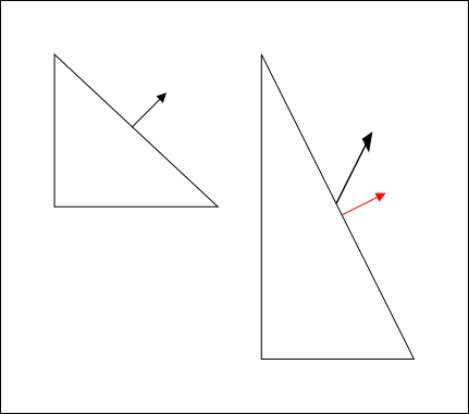
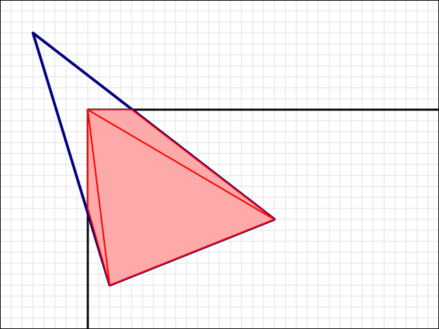
Additionally, as the r2 package does all lighting in eye space, it's necessary to transform the object space normal vectors given in mesh data to eye space. However, the usual model-view matrix will almost certainly contain some sort of translational component and possibly a scaling component. Normal vectors are not supposed to be translated; they represent directions! A non-uniform scale applied to an object will also deform the normal vectors, making them non-perpendicular to the surface they're associated with:
With the scaled triangle on the right, the normal vector is now not perpendicular to the surface (in addition to no longer being of unit length). The red vector indicates what the surface normal should be.
Therefore it's necessary to derive another 3x3 matrix known as the normal matrix from the model-view matrix that contains just the rotational component of the original matrix. The full derivation of this matrix is given in Mathematics for 3D Game Programming and Computer Graphics, Third Edition [4]. Briefly, the normal matrix is equal to the inverse transpose of the top left 3x3 elements of an arbitrary 4x4 model-view matrix.
In other rendering systems, eye space is sometimes referred to as camera space, or view space.
In the r2 package, eye space is represented by the R2SpaceEyeType.
Clip Space
Clip space is a homogeneous coordinate system in which OpenGL performs clipping of primitives (such as triangles). In OpenGL, clip space is effectively a left-handed coordinate system by default [7]. Intuitively, coordinates in eye space are transformed with a projection (normally either an orthographic or perspective projection) such that all vertices are projected into a homogeneous unit cube placed at the origin - clip space - resulting in four-dimensional (x, y, z, w) positions. Positions that end up outside of the cube are clipped (discarded) by dedicated clipping hardware, usually producing more triangles as a result.
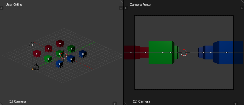
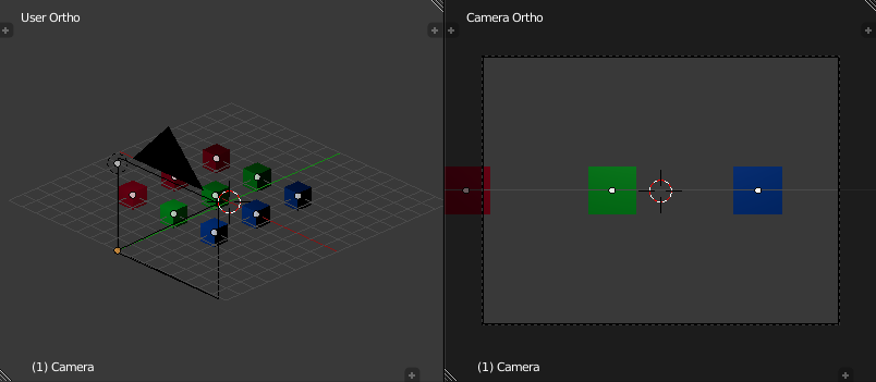
A projection effectively determines how objects in the three-dimensional scene are projected onto the two-dimensional viewing plane (a computer screen, in most cases) . A perspective projection transforms vertices such that objects that are further away from the viewing plane appear to be smaller than objects that are close to it, while an orthographic projection preserves the perceived sizes of objects regardless of their distance from the viewing plane.
Because eye space is a right-handed coordinate system by convention, but by default clip space is left-handed, the projection matrix used will invert the sign of the z component of any given point.
In the r2 package, the observer produces a 4x4 projection matrix. The projection matrix is passed, along with the model-view matrix, to the renderer's vertex shaders. As is normal in OpenGL, the vertex shader produces clip space coordinates which are then used by the hardware rasterizer to produce color fragments onscreen.
In the r2 package, clip space is represented by the R2SpaceClipType.
Normalized-Device Space
Normalized-device space is, by default, a left-handed [8] coordinate space in which clip space coordinates have been divided by their own w component (discarding the resulting w = 1 component in the process), yielding three dimensional coordinates. The range of values in the resulting coordinates are effectively normalized by the division to fall within the ranges [(-1, -1, -1), (1, 1, 1)] [9]. The coordinate space represents a simplifying intermediate step between having clip space coordinates and getting something projected into a two-dimensional image (screen space) for viewing.
The r2 package does not directly use or manipulate values in normalized-device space; it is mentioned here for completeness.
Screen Space
Screen space is, by default, a left-handed coordinate system representing the screen (or window) that is displaying the actual results of rendering. If the screen is of width w and height h, and the current depth range of the window is [n, f], then the range of values in screen space coordinates runs from [(0, 0, n), (w, h, f)]. The origin (0, 0, 0) is assumed to be at the bottom-left corner.
The depth range is actually a configurable value, but the r2 package keeps the OpenGL default. From the glDepthRange function manual page:
After clipping and division by w, depth coordinates range from -1 to 1,
corresponding to the near and far clipping planes. glDepthRange specifies a
linear mapping of the normalized depth coordinates in this range to window
depth coordinates. Regardless of the actual depth buffer implementation,
window coordinate depth values are treated as though they range from 0
through 1 (like color components). Thus, the values accepted by
glDepthRange are both clamped to this range before they are accepted.
The setting of (0,1) maps the near plane to 0 and the far plane to 1.
With this mapping, the depth buffer range is fully utilized.
As OpenGL, by default, specifies a depth range of [0, 1], the positive Z axis points away from the observer and so the coordinate system is left handed.
Meshes
Overview
A mesh is a collection of vertices that make up the triangles that define a polyhedral object, allocated on the GPU upon which the renderer is executing. In practical terms, a mesh is a pair (a, i), where a is an OpenGL vertex buffer object consisting of vertices, an i is an OpenGL element buffer object consisting of indices that describe how to draw the mesh as a series of triangles.
The contents of a are mutable, but mesh references are considered to be immutable.
Attributes
A mesh consists of vertices. A vertex can be considered to be a value of a record type, with the fields of the record referred to as the attributes of the vertex. In the r2 package, an array buffer containing vertex data is specified using the array buffer types from jcanephora. The jcanephora package allows programmers to specify the exact types of array buffers, allows for the full inspection of type information at runtime, including the ability to reference attributes by name, and allows for type-safe modification of the contents of array buffers using an efficient cursor interface.
Each attribute within an array buffer is assigned a numeric attribute index. A numeric index is an arbitrary number between (including) 0 and some OpenGL implementation-defined upper limit. On modern graphics hardware, OpenGL allows for at least 16 numeric attributes. The indices are used to create an association between fields in the array buffer and shader inputs. For the sake of sanity and consistency, it is the responsibility of rendering systems using OpenGL to establish conventions for the assignment of numeric attribute indices in shaders and array buffers [12]. For example, many systems state that attribute 0 should be of type vec4 and should represent vertex positions. Shaders simply assume that data arriving on attribute input 0 represents position data, and programmers are expected to create meshes where attribute 0 points to the field within the array that contains position data.
The r2 package uses the following conventions everywhere:
| Index | Type | Description |
|---|---|---|
| 0 | vec3 | The object-space position of the vertex |
| 1 | vec2 | The UV coordinates of the vertex |
| 2 | vec3 | The object-space normal vector of the vertex |
| 3 | vec4 | The tangent vector of the vertex |
Batched instances are expected to use the following additional conventions:
Types
In the r2 package, the given attribute conventions are specified by the R2AttributeConventions type.
Transforms
Overview
The ultimate purpose of a transform is to produce one or more matrices that can be combined with other matrices and then finally passed to a shader. The shader uses these matrices to transform vertices and normal vectors during the rendering of objects.
A transform is effectively responsible for producing a model matrix that transforms positions in object space to world space.
Instances
Overview
An instance is a renderable object. There are several types of instances available in the r2 package: single, batched, and billboarded.
Single
A single instance is the simplest type of instance available in the r2 package. A single instance is simply a pair (m, t), where m is a mesh, and t is a transform capable of transforming the object space coordinates of the vertices contained within m to world space.
Batched
A batched instance represents a group of (identical) renderable objects. The reason for the existence of batched instances is simple efficiency: On modern rendering hardware, rendering n single instances means submitting n draw calls to the GPU. As n becomes increasingly large, the overhead of the large number of draw calls becomes a bottleneck for rendering performance. A batched instance of size m allows for rendering a given mesh m times in a single draw call.
A batched instance of size n is a 3-tuple (m, b, t), where m is a mesh, b is a buffer of n 4x4 matrices allocated on the GPU, and t is an array of n transforms allocated on the CPU. For each i where 0 <= i < n, b[i] is the 4x4 model matrix produced from t[i]. The contents of b are typically recalculated and uploaded to the GPU once per rendering frame.
Billboarded
A billboarded instance is a further specialization of batched instances. Billboarding is the name given to a rendering technique where instead of rendering full 3D objects, simple 2D images of those objects are rendered instead using flat rectangles that are arranged such that they are always facing directly towards the observer.
A billboarded instance of size n is a pair (m, p), where m is a mesh [13], and p is a buffer of n world space positions allocated on the GPU.
Render Targets
Shaders
Interface And Calling Protocol
Every shader in the r2 package has an associated Java class. Each class may implement one of the interfaces that are themselves subtypes of the R2ShaderType interface. Each class is responsible for uploading parameters to the actual compiled GLSL shader on the GPU. Certain parameters, such as view matrices, the current size of the screen, etc, are only calculated during each rendering pass and therefore will be supplied to the shader classes at more or less the last possible moment. The calculated parameters are supplied via methods defined on the R2ShaderType subinterfaces, and implementations of the subinterfaces can rely on the methods being called in a very strict predefined order. For example, instances of type R2ShaderInstanceSingleUsableType will receive calls in exactly this order:
- First, onActivate will be called. It is the class's responsibility to activate the GLSL shader at this point.
- Then onReceiveViewValues will be called when the current view-specific values have been calculated.
- Now, for each material m that uses the current shader:
- onReceiveMaterialValues will be called once.
- For each instance i using that uses a material that uses the current shader, onReceiveInstanceTransformValues will be called, followed by onValidate.
The final onValidate call allows the shader to check that all of the required method calls have actually been made by the caller, and the method is permitted to throw R2ExceptionShaderValidationFailed if the caller makes a mistake at any point. The implicit promise is that callers will call all of the methods in the correct order and the correct number of times, and shaders are allowed to loudly complain if and when this does not happen.
Of course, actually requiring the programmer to manually implement all of the above for each new shader would be unreasonable and would just become a new source of bugs. The r2 provides abstract shader implementations to perform the run-time checks listed above without forcing the programmer to implement them all manually. The R2AbstractInstanceShaderSingle type, for example, implements the R2ShaderInstanceSingleUsableType interface and provides a few abstract methods that the programmer implements in order to upload parameters to the GPU. The abstract implementation enforces the calling protocol.
The calling protocol described both ensures that all shader parameters will be set and that the renderers themselves are insulated from the interfaces of actual GLSL shaders. Failing to set parameters, attempting to set parameters that no longer exist, or passing values of the wrong types to GLSL shaders is a common source of bugs in OpenGL programs and almost always results in either silent failure or corrupted visuals. The r2 package takes care to ensure that mistakes of that type are difficult to make.
Shader Modules
Although the GLSL shading language is anti-modular in the sense that it has one large namespace, the r2 package attempts to relieve some of the pain of shader management by delegating to the sombrero package. The sombrero package provides a preprocessor for shader code, allowing shader code to make use of #include directives. It also provides a system for publishing and importing modules full of shaders based internally on the standard Java ServiceLoader API. This allows users that want to write their own shaders to import much of the re-usable shader code from the r2 package into their own shaders without needing to do anything more than have the correct shader jar on the Java classpath [14].
As a simple example, if the user writing custom shaders wants to take advantage of the bilinear interpolation functions used in many r2 shaders, the following #include is sufficient:
#include <com.io7m.r2.shaders.core/R2Bilinear.h>

vec3 x = R2_bilinearInterpolate3(...);
The text com.io7m.r2.shaders.core is considered to be the module name, and the R2Bilinear.h name refers to that file within the module. The sombrero resolver maps the request to a concrete resource on the filesystem or in a jar file and returns the content for inclusion.
The r2 package also provides an interface, the R2ShaderPreprocessingEnvironmentType type, that allows constants to be set that will be exposed to shaders upon being preprocessed. Each shader stores an immutable snapshot of the environment used to preprocess it after successful compilation.
Shaders: Instance
Overview
An instance shader is a shader used to render the surfaces of instances. Depending on the context, this may mean rendering the surface attributes of the instances into a geometry buffer, forward rendering the instance directly to the screen (or
other image) , rendering only the depth of the surface, or perhaps not producing any output at all as shaders used simply for stencilling are permitted to do. Instance shaders are most often exposed to the programmer via materials.
Materials
A material is a pair (s, i, p) where p is a value of type m that represents a set of shader parameters, s is a shader that takes parameters of type m, and i is a unique identifier for the material. Materials primarily exist to facilitate batching: By assigning each material a unique identifier, the system can assume that two materials are the same if they have the same identifier, without needing to perform a relatively expensive structural equality comparison between the shaders and shader parameters.
Provided Shaders
Writing shaders is difficult. The programmer must be aware of an endless series of pitfalls inherent in the OpenGL API and the shading language. While the r2 package does allow users to write their own shaders, the intention has always been to provide a small set of general purpose shaders that cover the majority of the use cases in modern games and simulations. The instance shaders provided by default are:
| Shader | Description |
|---|---|
| R2SurfaceShaderBasicSingle | Basic textured surface with normal mapping, specular mapping, emission mapping, and conditional discarding based on alpha. |
| R2SurfaceShaderBasicReflectiveSingle | Basic textured surface with pseudo reflections from a cube map, normal mapping, specular mapping, emission mapping, and conditional discarding based on alpha. |
Types
In the r2 package, materials are instances of R2MaterialType. Geometry renderers primarily consume instances that are associated with values of the R2MaterialOpaqueSingleType and R2MaterialOpaqueBatchedType types. Instance shaders are instances of the R2ShaderInstanceSingleType and R2ShaderInstanceBatchedType types.
Shaders: Light
Overview
A light shader is a shader used to render the contributions of a light source. Light shaders in the r2 package are only used within the context of deferred rendering.
Stencils
Reserved Bits
The current stencil buffer layout used by the r2 package is as follows:
Bit 0 is used for light clip volumes.
Bits 1-2 are reserved for future use.
Allow Bit
The r2 package reserves a single bit in the current stencil buffer, known as the allow bit. In all subsequent rendering operations, a pixel may only be written if the corresponding allow bit in the stencil buffer is true.
The stencil buffer allow bits are populated via the use of a stencil renderer. The user specifies a series of instances whose only purpose is to either enable or disable the allow bit for each rendered pixel. Users may specify whether instances are positive or negative. Positive instances set the allow bit to true for each overlapped pixel, and negative instances set the allow bit to false for each overlapped pixel.
Lighting
Overview
The following sections of documentation attempt to describe the theory and implementation of lighting in the r2 package. All lighting in the package is dynamic- there is no support for precomputed lighting and all contributions from lights are recalculated every time a scene is rendered. Lighting is configured by adding instances of R2LightType to a scene.
Diffuse/Specular Terms
The light applied to a surface by a given light is divided into diffuse and specular terms [15]. The actual light applied to a surface is dependent upon the properties of the surface. Conceptually, the diffuse and specular terms are multiplied by the final color of the surface and summed. In practice, the materials applied to surfaces have control over how light is actually applied to the surface. For example, materials may include a specular map which is used to manipulate the specular term as it is applied to the surface. Additionally, if a light supports attenuation, then the diffuse and specular terms are scaled by the attenuation factor prior to being applied.
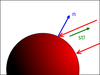
The diffuse term is modelled by Lambertian reflectance. Specifically, the amount of diffuse light reflected from a surface is given by diffuse in LightDiffuse.hs:
module LightDiffuse where

import qualified Color3
import qualified Direction
import qualified Normal
import qualified Spaces
import qualified Vector3f

diffuse ::  Direction.T Spaces.Eye -> Normal.T -> Color3.T -> Float -> Vector3f.T
diffuse stl n light_color light_intensity =
  let
    factor       = max 0.0 (Vector3f.dot3 stl n)
    light_scaled = Vector3f.scale light_color light_intensity
  in
Vector3f.scale light_scaled factorWhere stl is a unit length direction vector from the surface to the light source, n is the surface normal vector, light_color is the light color, and light_intensity is the light intensity. Informally, the algorithm determines how much diffuse light should be reflected from a surface based on how directly that surface points towards the light. When stl == n, Vector3f.dot3 stl n == 1.0, and therefore the light is reflected exactly as received. When stl is perpendicular to n (such that Vector3f.dot3 stl n == 0.0 ), no light is reflected at all. If the two directions are greater than 90° perpendicular, the dot product is negative, but the algorithm clamps negative values to 0.0 so the effect is the same.
The specular term is modelled either by Phong or Blinn-Phong reflection. The r2 package provides light shaders that provide both Phong and Blinn-Phong specular lighting and the user may freely pick between implementations. For the sake of simplicity, the rest of this documentation assumes that Blinn-Phong shading is being used. Specifically, the amount of specular light reflected from a surface is given by specularBlinnPhong in LightSpecular.hs:
module LightSpecular where

import qualified Color3
import qualified Direction
import qualified Normal
import qualified Reflection
import qualified Spaces
import qualified Specular
import qualified Vector3f

specularPhong :: Direction.T Spaces.Eye -> Direction.T Spaces.Eye -> Normal.T -> Color3.T -> Float -> Specular.T -> Vector3f.T
specularPhong stl view n light_color light_intensity (Specular.S surface_spec surface_exponent) =
  let
    reflection   = Reflection.reflection view n
    factor       = (max 0.0 (Vector3f.dot3 reflection stl)) ** surface_exponent
    light_raw    = Vector3f.scale light_color light_intensity
    light_scaled = Vector3f.scale light_raw factor
  in
    Vector3f.mult3 light_scaled surface_spec

specularBlinnPhong :: Direction.T Spaces.Eye -> Direction.T Spaces.Eye -> Normal.T -> Color3.T -> Float -> Specular.T -> Vector3f.T
specularBlinnPhong stl view n light_color light_intensity (Specular.S surface_spec surface_exponent) =
  let
    reflection   = Reflection.reflection view n
    factor       = (max 0.0 (Vector3f.dot3 reflection stl)) ** surface_exponent
    light_raw    = Vector3f.scale light_color light_intensity
    light_scaled = Vector3f.scale light_raw factor
  in
Vector3f.mult3 light_scaled surface_specWhere stl is a unit length direction vector from the surface to the light source, view is a unit length direction vector from the observer to the surface, n is the surface normal vector, light_color is the light color, light_intensity is the light intensity, surface_exponent is the specular exponent defined by the surface, and surface_spec is the surface specularity factor.
The specular exponent is a value, ordinarily in the range [0, 255], that controls how sharp the specular highlights appear on the surface. The exponent is a property of the surface, as opposed to being a property of the light. Low specular exponents result in soft and widely dispersed specular highlights (giving the appearance of a rough surface), while high specular exponents result in hard and focused highlights (giving the appearance of a polished surface). As an example, three models lit with progressively lower specular exponents from left to right ( 128, 32, and 8, respectively):
Attenuation
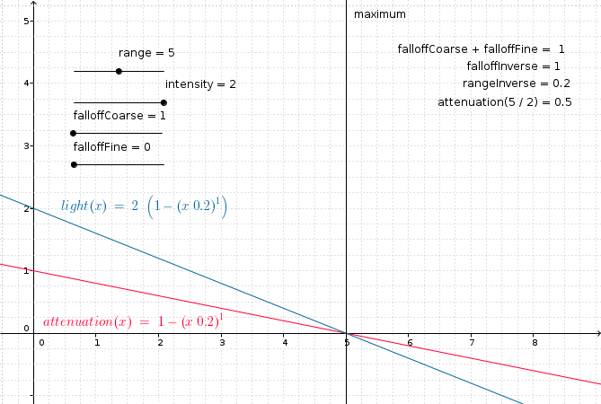
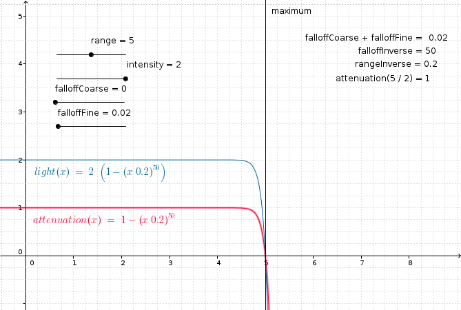
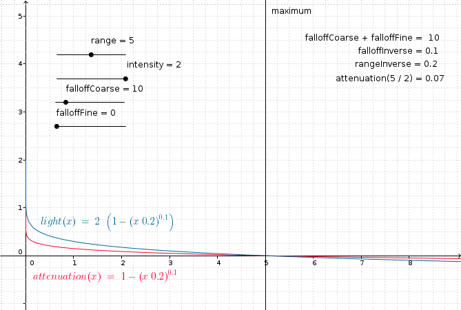
Attenuation is the property of the influence of a given light on a surface in inverse proportion to the distance from the light to the surface. In other words, for lights that support attenuation, the further a surface is from a light source, the less that surface will appear to be lit by the light. For light types that support attenuation, an attenuation factor is calculated based on a given inverse_maximum_range (where the maximum_range is a light-type specific positive value that represents the maximum possible range of influence for the light), a configurable inverse falloff value, and the current distance between the surface being lit and the light source. The attenuation factor is a value in the range [0.0, 1.0], with 1.0 meaning "no attenuation" and 0.0 meaning "maximum attenuation". The resulting attenuation factor is multiplied by the raw unattenuated light values produced for the light in order to produce the illusion of distance attenuation. Specifically:
module Attenuation where

attenuation_from_inverses :: Float -> Float -> Float -> Float
attenuation_from_inverses inverse_maximum_range inverse_falloff distance =
  max 0.0 (1.0 - (distance * inverse_maximum_range) ** inverse_falloff)

attenuation :: Float -> Float -> Float -> Float
attenuation maximum_range falloff distance =
  attenuation_from_inverses (1.0 / maximum_range) (1.0 / falloff) distance
Given the above definitions, a number of observations can be made.
If maximum_range == 0, then the inverse range is undefined, and therefore the results of lighting are undefined. The r2 package handles this case by raising an exception when the light is created.
If falloff == 0, then the inverse falloff is undefined, and therefore the results of lighting are undefined. The r2 package handles this case by raising an exception when the light is created.
As falloff decreases towards 0.0, then the attenuation curve remains at 1.0 for increasingly higher distance values before falling sharply to 0.0:
As falloff increases away from 0.0, then the attenuation curve decreases more for lower distance values:
Lighting: Directional
Overview
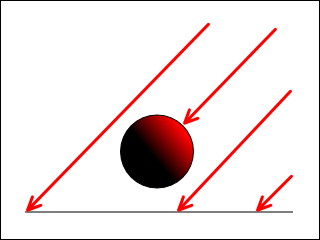
Directional lighting is the most trivial form of lighting provided by the r2 package. A directional light is a light that emits parallel rays of light in a given eye space direction. It has a color and an intensity, but does not have an origin and therefore is not attenuated over distance. It does not cause objects to cast shadows.
Application
The final light applied to the surface is given by directional (Directional.hs), where sr, sg, sb are the red, green, and blue channels, respectively, of the surface being lit. Note that the surface-to-light vector stl is simply the negation of the light direction.
module Directional where

import qualified Color4
import qualified Direction
import qualified LightDirectional
import qualified LightDiffuse
import qualified LightSpecular
import qualified Normal
import qualified Position3
import qualified Spaces
import qualified Specular
import qualified Vector3f
import qualified Vector4f

directional :: Direction.T Spaces.Eye -> Normal.T -> Position3.T Spaces.Eye -> LightDirectional.T -> Specular.T -> Color4.T -> Vector3f.T
directional view n position light specular (Vector4f.V4 sr sg sb _) =
  let
    stl             = Vector3f.normalize (Vector3f.negation position)
    light_color     = LightDirectional.color light
    light_intensity = LightDirectional.intensity light
    light_d         = LightDiffuse.diffuse stl n light_color light_intensity
    light_s         = LightSpecular.specularBlinnPhong stl view n light_color light_intensity specular
    lit_d           = Vector3f.mult3 (Vector3f.V3 sr sg sb) light_d
    lit_s           = Vector3f.add3 lit_d light_s
  in
    lit_s
Types
Directional lights are represented in the r2 package by the R2LightDirectionalScreenSingle type.
Lighting: Spherical
Overview
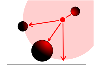
A spherical light in the r2 package is a light that emits rays of light in all directions from a given origin specified in eye space up to a given maximum radius.
The term spherical comes from the fact that the light has a defined radius. Most rendering systems instead use point lights that specify multiple attenuation constants to control how light is attenuated over distance. The problem with this approach is that it requires solving a quadratic equation to determine a minimum bounding sphere that can contain the light. Essentially, the programmer/artist is forced to determine "at which radius does the contribution from this light effectively reach zero?". With spherical lights, the maximum radius is declared up front, and a single falloff value is used to determine the attenuation curve within that radius. This makes spherical lights more intuitive to use: The programmer/artist simply places a sphere within the scene and knows exactly from the radius which objects are lit by it. It also means that bounding light volumes can be trivially constructed from unit spheres by simply scaling those spheres by the light radius, when performing deferred rendering.
Application
The final light applied to the surface is given by spherical (Spherical.hs), where sr, sg, sb are the red, green, and blue channels, respectively, of the surface being lit. The surface-to-light vector stl is calculated by normalizing the negation of the difference between the the current eye space surface_position and the eye space origin of the light.
module Spherical where

import qualified Attenuation
import qualified Color4
import qualified Direction
import qualified LightDiffuse
import qualified LightSpecular
import qualified LightSpherical
import qualified Normal
import qualified Position3
import qualified Specular
import qualified Spaces
import qualified Vector3f
import qualified Vector4f

spherical :: Direction.T Spaces.Eye -> Normal.T -> Position3.T Spaces.Eye -> LightSpherical.T -> Specular.T -> Color4.T -> Vector3f.T
spherical view n surface_position light specular (Vector4f.V4 sr sg sb _) =
  let
    position_diff   = Position3.sub3 surface_position (LightSpherical.origin light)
    stl             = Vector3f.normalize (Vector3f.negation position_diff)
    distance        = Vector3f.magnitude (position_diff)
    attenuation     = Attenuation.attenuation (LightSpherical.radius light) (LightSpherical.falloff light) distance
    light_color     = LightSpherical.color light
    light_intensity = LightSpherical.intensity light
    light_d         = LightDiffuse.diffuse stl n light_color light_intensity
    light_s         = LightSpecular.specularBlinnPhong stl view n light_color light_intensity specular
    light_da        = Vector3f.scale light_d attenuation
    light_sa        = Vector3f.scale light_s attenuation
    lit_d           = Vector3f.mult3 (Vector3f.V3 sr sg sb) light_da
    lit_s           = Vector3f.add3 lit_d light_sa
  in
    lit_s
Lighting: Projective
- 2.15.1. Overview
- 2.15.2. Algorithm
- 2.15.3. Back projection
- 2.15.4. Clamping
- 2.15.5. Attenuation
- 2.15.6. Application
Overview
A projective light in the r2 package is a light that projects a texture onto the scene from a given origin specified in eye space up to a given maximum radius. Projective lights are the only types of lights in the r2 package that are able to project shadows.
Algorithm
At a basic level, a projective light performs the same operations that occur when an ordinary 3D position is projected onto the screen during rendering. During normal rendering, a point p given in world space is transformed to eye space given the current camera's view matrix, and is then transformed to clip space using the current camera's projection matrix. During rendering of a scene lit by a projective light, a given point q in the scene is transformed back to world space given the current camera's inverse view matrix, and is then transformed to eye space from the point of view of the light (subsequently referred to as light eye space) using the light's view matrix. Finally, q is transformed to clip space from the point of view of the light (subsequently referred to as light clip space) using the light's projection matrix. It should be noted (in order to indicate that there is nothing unusual about the light's view or projection matrices) that if the camera and light have the same position, orientation, scale, and projection, then the resulting transformed values of q and p are identical. The resulting transformed value of q is mapped from the range [(-1, -1, -1), (1, 1, 1)] to [(0, 0, 0), (1, 1, 1)], and the resulting coordinates are used to retrieve a texel from the 2D texture associated with the light.
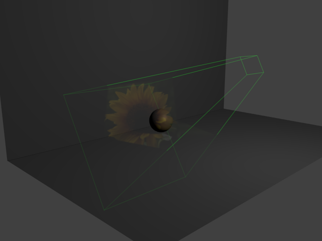
Intuitively, an ordinary perspective projection will cause the light to appear to take the shape of a frustum:
There are two issues with the projective lighting algorithm that also have to be solved: back projection and clamping.
Back projection
The algorithm described above will produce a so-called dual or back projection. In other words, the texture will be projected along the view direction of the camera, but will also be projected along the negative view direction [17]. The visual result is that it appears that there are two projective lights in the scene, oriented in opposite directions. As mentioned previously, given the typical projection matrix, the w component of a given clip space position is the negation of the eye space z component. Because it is assumed that the observer is looking towards the negative z direction, all positions that are in front of the observer must have positive w components. Therefore, if w is negative, then the position is behind the observer. The standard fix for this problem is to check to see if the w component of the light-clip space coordinate is negative, and simply return a pure black color (indicating no light contribution) rather than sampling from the projected texture.
Clamping
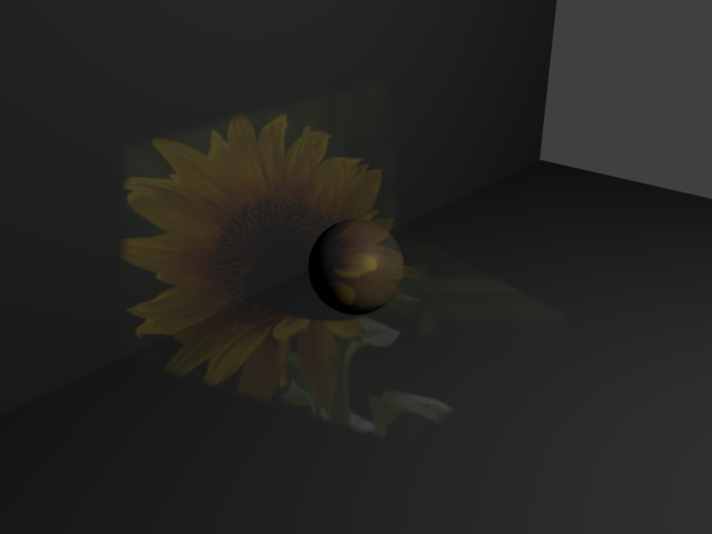
The algorithm described above takes an arbitrary point in the scene and projects it from the point of view of the light. There is no guarantee that the point actually falls within the light's view frustum (although this is mitigated slightly by the r2 package's use of light volumes for deferred rendering), and therefore the calculated texture coordinates used to sample from the projected texture are not guaranteed to be in the range [(0, 0), (1, 1)]. In order to get the intended visual effect, the texture used must be set to clamp-to-edge and have black pixels on all of the edges of the texture image, or clamp-to-border with a black border color. Failing to do this can result in strange visual anomalies, as the texture will be unexpectedly repeated or smeared across the area outside of the intersection between the light volume and the receiving surface:
The r2 package will raise an exception if a non-clamped texture is assigned to a projective light.
Application
The final light applied to the surface is given by projective in Projective.hs, where sr, sg, sb are the red, green, and blue channels, respectively, of the surface being lit. The surface-to-light vector stl is calculated by normalizing the negation of the difference between the the current eye space surface_position and the eye space origin of the light.
module Projective where

import qualified Attenuation
import qualified Color3
import qualified Color4
import qualified Direction
import qualified LightDiffuse
import qualified LightSpecular
import qualified LightProjective
import qualified Normal
import qualified Position3
import qualified Specular
import qualified Spaces
import qualified Vector3f
import qualified Vector4f

projective :: Direction.T Spaces.Eye -> Normal.T -> Position3.T Spaces.Eye -> LightProjective.T -> Specular.T -> Float -> Color3.T -> Color4.T -> Vector3f.T
projective view n surface_position light specular shadow texture (Vector4f.V4 sr sg sb _) =
  let
    position_diff   = Position3.sub3 surface_position (LightProjective.origin light)
    stl             = Vector3f.normalize (Vector3f.negation position_diff)
    distance        = Vector3f.magnitude (position_diff)
    attenuation_raw = Attenuation.attenuation (LightProjective.radius light) (LightProjective.falloff light) distance
    attenuation     = attenuation_raw * shadow
    light_color     = Vector3f.mult3 (LightProjective.color light) texture
    light_intensity = LightProjective.intensity light
    light_d         = LightDiffuse.diffuse stl n light_color light_intensity
    light_s         = LightSpecular.specularBlinnPhong stl view n light_color light_intensity specular
    light_da        = Vector3f.scale light_d attenuation
    light_sa        = Vector3f.scale light_s attenuation
    lit_d           = Vector3f.mult3 (Vector3f.V3 sr sg sb) light_da
    lit_s           = Vector3f.add3 lit_d light_sa
  in
    lit_s
The given shadow factor is a value in the range [0, 1], where 0 indicates that the lit point is fully in shadow for the current light, and 1 indicates that the lit point is not in shadow. This is calculated for variance shadows and is assumed to be 1 for lights without shadows. As can be seen, a value of 0 has the effect of fully attenuating the light.
The color denoted by texture is assumed to have been sampled from the projected texture. Assuming the eye space position being shaded p, the matrix to get from eye space to light-clip space is given by The final light applied to the surface is given by projective_matrix in ProjectiveMatrix.hs:
module ProjectiveMatrix where

import qualified Matrix4f

projective_matrix :: Matrix4f.T -> Matrix4f.T -> Matrix4f.T -> Matrix4f.T
projective_matrix camera_view light_view light_projection =
  case Matrix4f.inverse camera_view of
    Just cv -> Matrix4f.mult (Matrix4f.mult light_projection light_view) cv
    Nothing -> undefined -- A view matrix is always invertible
Shadows
Overview
Because the r2 package implements local illumination, it is necessary to associate shadows with those light sources capable of projecting them (currently only projective lights). The r2 package currently only supports variance shadow mapping. So-called mapped shadows allow efficient per-pixel shadows to be calculated with varying degrees of visual quality.
Shadow Geometry
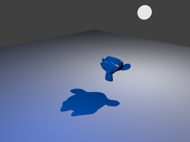
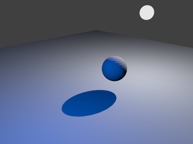
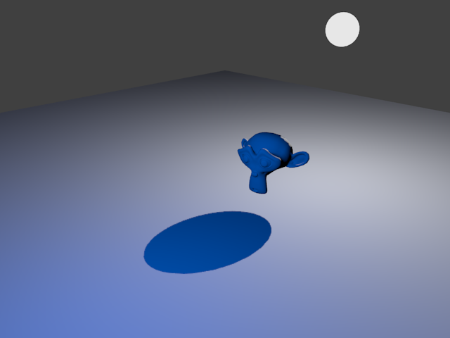
Because the system requires the programmer to explicitly and separately state that an opaque instance is visible in the scene, and that an opaque instance is casting a shadow, it becomes possible to effectively specify different shadow geometry for a given instance. As an example, a very complex and high resolution mesh may still have the silhouette of a simple sphere, and therefore the user can separately add the high resolution mesh to a scene as a visible instance, but add a low resolution version of the mesh as an invisible shadow-casting instance with the same transform. As a rather extreme example, assuming a high resolution mesh m0 added to the scene as both a visible instance and a shadow caster:
A low resolution mesh m1 added to the scene as both a visible instance and shadow caster:
Now, with m1 added as only a shadow caster, and m0 added as only a visible instance:
Using lower resolution geometry for shadow casters can lead to efficiency gains on systems where vertex processing is expensive.
Shadows: Variance Mapping
Overview
Variance shadow mapping is a technique that can give attractive soft-edged shadows. Using the same view and projection matrices used to apply projective lights, a depth-variance image of the current scene is rendered, and those stored depth distribution values are used to determine the probability that a given point in the scene is in shadow with respect to the current light.
The algorithm implemented in the r2 package is described in GPU Gems 3, which is a set of improvements to the original variance shadow mapping algorithm by William Donnelly and Andrew Lauritzen. The r2 package implements all of the improvements to the algorithm except summed area tables. The package also provides optional box blurring of shadows as described in the chapter.
Algorithm
Prior to actually rendering a scene, shadow maps are generated for all shadow-projecting lights in the scene. A shadow map for variance shadow mapping, for a light k, is a two-component red/green image of all of the shadow casters associated with k in the visible set. The image is produced by rendering the instances from the point of view of k. The red channel of each pixel in the image represents the logarithmic depth of the closest surface at that pixel, and the green channel represents the depth squared (literally depth * depth ). For example:
Then, when actually applying lighting during rendering of the scene, a given eye space position p is transformed to light-clip space and then mapped to the range [(0, 0, 0), (1, 1, 1)] in order to sample the depth and depth squared values (d, ds) from the shadow map (as with sampling from a projected texture with projective lighting).
As stated previously, the intent of variance shadow mapping is to essentially calculate the probability that a given point is in shadow. A one-tailed variant of Chebyshev's inequality is used to calculate the upper bound u on the probability that, given (d, ds), a given point with depth t is in shadow:
module ShadowVarianceChebyshev0 where

chebyshev :: (Float, Float) -> Float -> Float
chebyshev (d, ds) t =
  let p        = if t <= d then 1.0 else 0.0
      variance = ds - (d * d)
      du       = t - d
      p_max    = variance / (variance + (du * du))
  in max p p_max

factor :: (Float, Float) -> Float -> Float
factor = chebyshev
One of the improvements suggested to the original variance shadow algorithm is to clamp the minimum variance to some small value (the r2 package uses 0.00002 by default, but this is configurable on a per-shadow basis). The equation above becomes:
module ShadowVarianceChebyshev1 where

data T = T {
  minimum_variance :: Float
} deriving (Eq, Show)

chebyshev :: (Float, Float) -> Float -> Float -> Float
chebyshev (d, ds) min_variance t =
  let p        = if t <= d then 1.0 else 0.0
      variance = max (ds - (d * d)) min_variance
      du       = t - d
      p_max    = variance / (variance + (du * du))
  in max p p_max

factor :: T -> (Float, Float) -> Float -> Float
factor shadow (d, ds) t =
  chebyshev (d, ds) (minimum_variance shadow) t
The above is sufficient to give shadows that are roughly equivalent in visual quality to basic shadow mapping with the added benefit of being generally better behaved and with far fewer artifacts. However, the algorithm can suffer from light bleeding, where the penumbrae of overlapping shadows can be unexpectedly bright despite the fact that the entire area should be in shadow. One of the suggested improvements to reduce light bleeding is to modify the upper bound u such that all values below a configurable threshold are mapped to zero, and values above the threshold are rescaled to map them to the range [0, 1]. The original article suggests a linear step function applied to u:
module ShadowVarianceChebyshev2 where

data T = T {
  minimum_variance :: Float,
  bleed_reduction  :: Float
} deriving (Eq, Show)

chebyshev :: (Float, Float) -> Float -> Float -> Float
chebyshev (d, ds) min_variance t =
  let p        = if t <= d then 1.0 else 0.0
      variance = max (ds - (d * d)) min_variance
      du       = t - d
      p_max    = variance / (variance + (du * du))
  in max p p_max

clamp :: Float -> (Float, Float) -> Float
clamp x (lower, upper) = max (min x upper) lower

linear_step :: Float -> Float -> Float -> Float
linear_step lower upper x = clamp ((x - lower) / (upper - lower)) (0.0, 1.0)

factor :: T -> (Float, Float) -> Float -> Float
factor shadow (d, ds) t =
  let u = chebyshev (d, ds) (minimum_variance shadow) t in
    linear_step (bleed_reduction shadow) 1.0 u
The amount of light bleed reduction is adjustable on a per-shadow basis.
To reduce problems involving numeric inaccuracy, the original article suggests the use of 32-bit floating point textures in depth variance maps. The r2 package allows 16-bit or 32-bit textures, configurable on a per-shadow basis.
Finally, as mentioned previously, the r2 package allows both optional box blurring and mipmap generation for shadow maps. Both blurring and mipmapping can reduce aliasing artifacts, with the former also allowing the edges of shadows to be significantly softened as a visual effect:
Advantages
The main advantage of variance shadow mapping is that they can essentially be thought of as much better behaved version of basic shadow mapping that just happen to have built-in softening and filtering. Variance shadows typically require far less in the way of scene-specific tuning to get good results.
Disadvantages
One disadvantage of variance shadows is that for large shadow maps, filtering quickly becomes a major bottleneck. On reasonably old hardware such as the Radeon 4670, one 8192x8192 shadow map with two 16-bit components takes too long to filter to give a reliable 60 frames per second rendering rate. Shadow maps of this size are usually used to simulate the influence of the sun over large outdoor scenes.
Types
Variance mapped shadows are represented by the R2ShadowDepthVarianceType type, and can be associated with projective lights.
Rendering of depth-variance images is handled by implementations of the R2ShadowMapRendererType type.
Deferred Rendering
Overview
Deferred rendering is a rendering technique where all of the opaque objects in a given scene are rendered into a series of buffers, and then lighting is applied to those buffers in screen space. This is in contrast to forward rendering, where all lighting is applied to objects as they are rendered.
One major advantage of deferred rendering is a massive reduction in the number of shaders required (traditional forward rendering requires s * l shaders, where s is the number of different object surface types in the scene, and l is the number of different light types). In contrast, deferred rendering requires s + l shaders, because surface and lighting shaders are applied separately.
Traditional forward rendering also suffers severe performance problems as the number of lights in the scene increases, because it is necessary to recompute all of the surface attributes of an object each time a light is applied. In contrast, deferred rendering calculates all surface attributes of all objects once, and then reuses them when lighting is applied.
However, deferred renderers are usually incapable of rendering translucent objects. The deferred renderer in the r2 package is no exception, and a separate set of renderers are provided to render translucent objects.
Due to the size of the subject, the deferred rendering infrastructure in the r2 package is described in several sections. The rendering of opaque geometry is described in the Geometry section, the subsequent lighting of that geometry is described in the Lighting section. The details of the position reconstruction algorithm, an algorithm utterly fundamental to deferred rendering, is described in Position Reconstruction.
Deferred Rendering: Geometry
- 2.19.1. Overview
- 2.19.2. Groups
- 2.19.3. Geometry Buffer
- 2.19.4. Algorithm
- 2.19.5. Ordering/Batching
- 2.19.6. Normal Compression
Overview
The first step in deferred rendering involves rendering all opaque instances in the current scene to a geometry buffer. This populated geometry buffer is then primarily used in later stages to calculate lighting, but can also be used to implement effects such as screen-space ambient occlusion and emission.
In the r2 package, the primary implementation of the deferred geometry rendering algorithm is the R2GeometryRenderer type.
Groups
Groups are a simple means to constrain the contributions of sets of specific light sources to sets of specific rendered instances. Instances and lights are assigned a group number in the range [1, 15]. If the programmer does not explicitly assign a number, the number 1 is assigned automatically. During rendering, the group number of each rendered instance is written to the stencil buffer. Then, when the light contribution is calculated for a light with group number n, only those pixels that have a corresponding value of n in the stencil buffer are allowed to be modified.
Geometry Buffer
A geometry buffer is a render target in which the surface attributes of objects are stored prior to being combined with the contents of a light buffer to produce a lit image.
One of the main implementation issues in any deferred renderer is deciding which surface attributes (such as position, albedo, normals, etc) to store and which to reconstruct. The more attributes that are stored, the less work is required during rendering to reconstruct those values. However, storing more attributes requires a larger geometry buffer and more memory bandwidth to actually populate that geometry buffer during rendering. The r2 package leans towards having a more compact geometry buffer and doing slightly more reconstruction work during rendering.
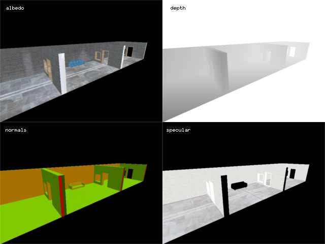
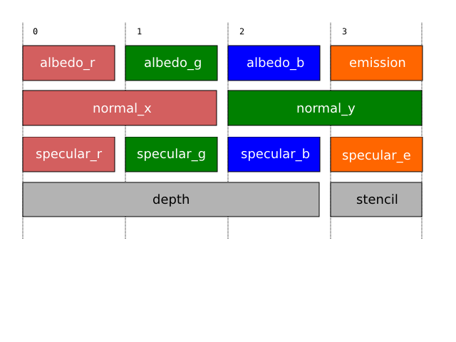
The r2 package explicitly stores the albedo, normals, emission level, and specular color of surfaces. Additionally, the depth buffer is sampled to recover the depth of surfaces. The eye-space positions of surfaces are recovered via an efficient position reconstruction algorithm which uses the current viewing projection and logarithmic depth value as input. In order to reduce the amount of storage required, three-dimensional eye-space normal vectors are stored compressed as two 16 half-precision floating point components via a simple mapping. This means that only 32 bits are required to store the vectors, and very little precision is lost. The precise format of the geometry buffer is as follows:
The albedo_r, albedo_g, and albedo_b components correspond to the red, green, and blue components of the surface, respectively. The emission component refers to the surface emission level. The normal_x and normal_y components correspond to the two components of the compressed surface normal vector. The specular_r, specular_g, and specular_b components correspond to the red, green, and blue components of the surface specularity. Surfaces that will not receive specular highlights simply have 0 for each component. The specular_e component holds the surface specular exponent divided by 256.
In the r2 package, geometry buffers are instances of R2GeometryBufferType.
Algorithm
An informal description of the geometry rendering algorithm as implemented in the r2 package is as follows:
- Set the current render target to a geometry buffer b.
- Enable writing to the depth and stencil buffers, and enable stencil testing. Enable depth testing such that only pixels with a depth less than or equal to the current depth are touched.
- For each group g:
- Configure stencil testing such that only pixels with the allow bit enabled are touched, and configure stencil writing such that the index of g is recorded in the stencil buffer.
- For each instance o in g:
- Render the surface albedo, eye space normals, specular color, and emission level of o into b. Normal mapping is performed during rendering, and if o does not have specular highlights, then a pure black (zero intensity) specular color is written. Effects such as environment mapping are considered to be part of the surface albedo and so are performed in this step.
Ordering/Batching
Due to the use of depth testing, the geometry rendering algorithm is effectively order independent: Instances can be rendered in any order and the final image will always be the same. However, there are efficiency advantages in rendering instances in a particular order. The most efficient order of rendering is the one that minimizes internal OpenGL state changes. NVIDIA's Beyond Porting presentation gives the relative cost of OpenGL state changes, from most expensive to least expensive, as [18]:
- Render target changes: 60,000/second
- Program bindings: 300,000/second
- Texture bindings: 1,500,000/second
- Vertex format (exact cost unspecified)
- UBO bindings (exact cost unspecified)
- Vertex Bindings (exact cost unspecified)
- Uniform Updates: 10,000,000/second
Therefore, it is beneficial to order rendering operations such that the most expensive state changes happen the least frequently.
The R2SceneOpaquesType type provides a simple interface that allows the programmer to specify instances without worrying about ordering concerns. When all instances have been submitted, they will be delivered to a given consumer (typically a geometry renderer) via the opaquesExecute method in the order that would be most efficient for rendering. Typically, this means that instances are first batched by shader, because switching programs is the second most expensive type of render state change. The shader-batched instances are then batched by material, in order to reduce the number of uniform updates that need to occur per shader.
Normal Compression
The r2 package uses a Lambert azimuthal equal-area projection to store surface normal vectors in two components instead of three. This makes use of the fact that normalized vectors represent points on the unit sphere. The mapping from normal vectors to two-dimensional spheremap coordinates is given by compress NormalCompress.hs:
module NormalCompress where

import qualified Vector3f
import qualified Vector2f
import qualified Normal

compress :: Normal.T -> Vector2f.T
compress n =
  let p = sqrt ((Vector3f.z n * 8.0) + 8.0)
      x = (Vector3f.x n / p) + 0.5
      y = (Vector3f.y n / p) + 0.5
in Vector2f.V2 x yThe mapping from two-dimensional spheremap coordinates to normal vectors is given by decompress NormalDecompress.hs:
module NormalDecompress where

import qualified Vector3f
import qualified Vector2f
import qualified Normal

decompress :: Vector2f.T -> Normal.T
decompress v =
  let fn = Vector2f.V2 ((Vector2f.x v * 4.0) - 2.0) ((Vector2f.y v * 4.0) - 2.0)
      f  = Vector2f.dot2 fn fn
      g  = sqrt (1.0 - (f / 4.0))
      x  = (Vector2f.x fn) * g
      y  = (Vector2f.y fn) * g
      z  = 1.0 - (f / 2.0)
in Vector3f.V3 x y zDeferred Rendering: Lighting
Overview
The second step in deferred rendering involves rendering the light contributions of all light sources within a scene to a light buffer. The rendering algorithm requires sampling from a populated geometry buffer.
Light Buffer
A light buffer is a render target in which the light contributions of all light sources are summed in preparation for being combined with the surface albedo of a geometry buffer to produce a lit image.
A light buffer consists of a 32-bit RGBA diffuse image and a 32-bit RGBA specular image. Currently, the alpha channels of both images are unused and exist solely because OpenGL 3.3 does not provide a color-renderable 24-bit RGB format.
The r2 package offers the ability to disable specular lighting entirely if it is not needed, and so light buffer implementations provide the ability to avoid allocating an image for specular contributions if they will not be calculated.
In the r2 package, light buffers are instances of R2LightBufferType.
Light Clip Volumes
A light clip volume is a means of constraining the contributions of groups of light sources to a provided volume.
Because, like most renderers, the r2 package implements so-called local illumination, lights that do not have explicit shadow mapping enabled are able to bleed through solid objects:
Enabling shadow mapping for every single light source would be prohibitively expensive [3], but for some scenes, acceptable results can be achieved by simply preventing the light source from affecting pixels outside of a given clip volume.
The technique is implemented using the stencil buffer, using a single light clip volume bit.
- Disable depth writing, and enable depth testing using the standard less-than-or-equal-to depth function is used.
- For each light clip volume v:
- Clear the light clip volume bit in the stencil buffer.
- Configure stencil testing such that the stencil test always passes.
- Configure stencil writing such that:
- Only the light clip volume bit can be written.
- Pixels that fail the depth test will invert the value of the light clip volume bit (GL_INVERT).
- Pixels that pass the depth test leave the value of the light clip volume bit untouched.
- Pixels that pass the stencil test leave the value of the light clip volume bit untouched.
- Render both the front and back faces of v.
- Configure stencil testing such that only those pixels with both the allow bit and light clip volume bit set will be touched.
- Render all of the light sources associated with v.
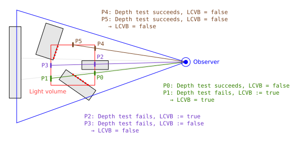
The reason the algorithm works can be inferred from the following diagram:
In the diagram, the grey polygons represent the already-rendered depths of the scene geometry [19]. If a point is inside or behind (from the perspective of the observer) one of the polygons, then the depth of the point is considered to be greater than the scene geometry.
In the diagram, when rendering the front face of the light volume at point P0, the depth of the light volume face at P0 is less than the current scene depth, and so the depth test succeeds and the light clip volume bit is not touched. When rendering the back face of the light volume at point P1, the depth of the light volume face at P1 is greater than the current scene depth so the depth test fails, and the light clip volume bit is inverted, setting it to true. This means that the scene geometry along that view ray is inside the light clip volume.
In the diagram, when rendering the front face of the light volume at point P2, the depth of the light volume face at P2 is greater than the current scene depth, and so the depth test fails and the light clip volume bit is inverted, setting it to true. When rendering the back face of the light volume at point P3, the depth of the light volume face at P3 is greater than the current scene depth, so the depth test fails and the light clip volume bit is inverted again, setting it to false. This means that the scene geometry along that view ray is outside the light clip volume.
In the diagram, when rendering the front face of the light volume at point P4, the depth of the light volume face at P4 is less than the current scene depth, and so the depth test succeeds and the light clip volume bit is not touched. When rendering the back face of the light volume at point P5, the depth of the light volume face at P5 is less than the current scene depth, and so the depth test succeeds and the light clip volume bit is not touched. Because the light clip volume bit is false by default and is not modified, this results in the scene geometry along that view ray being considered to be outside the light clip volume.
Given the initial depth buffer from an example scene:
After rendering a cuboid-shaped light volume that is intended to constrain the contributions of a light source to a single area, all pixels that fell within the clip volume have the light clip volume bit set:
Then, after rendering the light contribution of the constrainted light, the light contribution becomes:
No L-Buffer
The r2 package also provides basic support for rendering lit images directly without the use of an intermediate light buffer. This can save greatly on memory bandwidth if no intermediate processing of light buffers is required. In order to achieve this, light shaders must be preprocessed such that the output of the generated code is a lit image rather than simply the light contribution. Doing this is simple: Simply set R2_LIGHT_SHADER_OUTPUT_TARGET_DEFINE to R2_LIGHT_SHADER_OUTPUT_TARGET_IBUFFER in the shading environment prior to compiling any light shaders. The r2 renderer implementations perform simple run-time checks to ensure that light shaders have been compiled to support the current output type, so the programmer will be notified if they try to render directly to an image but fail to make the above configuration change.
Types
In the r2 package, the primary implementation of the deferred light rendering algorithm is the R2LightRenderer type.
Deferred Rendering: Position Reconstruction
- 2.21.1. Overview
- 2.21.2. Recovering Eye space Z
- 2.21.3. Recovering Eye space Z (Logarithmic depth encoding)
- 2.21.4. Recovering Eye space Z (Screen space depth encoding)
- 2.21.5. Recovering Eye space Position
- 2.21.6. Implementation
Overview
Applying lighting during deferred rendering is primarily a screen space technique. When the visible opaque objects have been rendered into the geometry buffer, the original eye space positions of all of the surfaces that resulted in visible fragments in the scene are lost (unless explicitly saved into the geometry buffer). However, given the knowledge of the projection that was used to render the scene (such as perspective or orthographic), it's possible to reconstruct the original eye space position of the surfaces that produced each of the fragments in the geometry buffer.
Specifically then, for each fragment f in the geometry buffer for which lighting is being applied, a position reconstruction algorithm attempts to reconstruct surface_eye - the eye space position of the surface that produced f - using the screen space position of the current light volume fragment position = (screen_x, screen_y) and some form of depth value (such as the screen space depth of f ).
Position reconstruction is a fundamental technique in deferred rendering, and there are a practically unlimited number of ways to reconstruct eye space positions for fragments, each with various advantages and disadvantages. Some rendering systems actually store the eye space position of each fragment in the geometry buffer, meaning that reconstructing positions means simply reading a value directly from a texture. Some systems store only a normalized eye space depth value in a separate texture: The first step of most position reconstruction algorithms is to compute the original eye space Z value of a fragment, so having this value computed during the population of the geometry buffer reduces the work performed later. Storing an entire eye space position into the geometry buffer is obviously the simplest and requires the least reconstruction work later on, but is costly in terms of memory bandwidth: Storing a full eye space position requires an extra 4 * 4 = 16 bytes of storage per fragment (four 32-bit floating point values). As screen resolutions increase, the costs can be prohibitive. Storing a normalized depth value requires only a single 32-bit floating point value per fragment but even this can be too much on less capable hardware. Some algorithms take advantage of the fact that most projections used to render scenes are perspective projections. Some naive algorithms use the full inverse of the current projection matrix to reconstruct eye space positions having already calculated clip space positions.
The algorithm that the r2 package uses for position reconstruction is generalized to handle both orthographic and perspective projections, and uses only the existing logarithmic depth values that were written to the depth buffer during scene rendering. This keeps the geometry buffer compact, and memory bandwidth requirements comparatively low. The algorithm works with symmetric and asymmetric viewing frustums, but will only work with near and far planes that are parallel to the screen.
The algorithm works in two steps: Firstly, the original eye space Z value of the fragment in question is recovered, and then this Z value is used to recover the full eye space position.
Recovering Eye space Z
During rendering of arbitrary scenes, vertices specified in object space are transformed to eye space, and the eye space coordinates are transformed to clip space with a projection matrix. The resulting 4D clip space coordinates are divided by their own w components, resulting in normalized-device space coordinates. These normalized-device space coordinates are then transformed to screen space by multiplying by the current viewport transform. The transitions from clip space to screen space are handled automatically by the graphics hardware.
The first step required is to recover the original eye space Z value of f. This involves sampling a depth value from the current depth buffer. Sampling from the depth buffer is achieved as with any other texture: A particular texel is addressed by using coordinates in the range [(0, 0), (1, 1)]. The r2 package currently assumes that the size of the viewport is the same as that of the framebuffer (width, height) and that the bottom left corner of the viewport is positioned at (0, 0) in screen space. Given the assumption on the position and size of the viewport, and assuming that the screen space position of the current light volume fragment being shaded is position = (screen_x, screen_y), the texture coordinates (screen_uv_x, screen_uv_y) used to access the current depth value are given by:
module ScreenToTexture where

import qualified Vector2f

screen_to_texture :: Vector2f.T -> Float -> Float -> Vector2f.T
screen_to_texture position width height =
  let u = (Vector2f.x position) / width
      v = (Vector2f.y position) / height
  in Vector2f.V2 u v
Intuitively, (screen_uv_x, screen_uv_y) = (0, 0) when the current screen space position is the bottom-left corner of the screen, (screen_uv_x, screen_uv_y) = (1, 1) when the current screen space position is the top-right corner of the screen, and (screen_uv_x, screen_uv_y) = (0.5, 0.5) when the current screen space position is the exact center of the screen.
Originally, the spiritual ancestor of the r2 package, r1, used a standard depth buffer and so recovering the eye space Z value required a slightly different method compared to the steps required for the logarithmic depth encoding that the r2 package uses. For historical reasons and for completeness, the method to reconstruct an eye space Z value from a traditional screen space depth value is given in the section on screen space depth encoding.
Recovering Eye space Z (Logarithmic depth encoding)
The r2 package uses a logarithmic depth buffer. Depth values sampled from any depth buffer produced by the package can be transformed to a negated eye space Z value by with a simple decoding equation.
Recovering Eye space Z (Screen space depth encoding)
Note: This section is for completeness and historical interest. Please skip ahead to the section on eye space position reconstruction if you are not interested.
Assuming a screen space depth value screen_depth sampled from the depth buffer at (screen_uv_x, screen_uv_y), it's now necessary to transform the depth value back into normalized-device space. In OpenGL, screen space depth values are in the range [0, 1] by default, with 0 representing the near plane and 1 representing the far plane. However, in OpenGL, normalized-device space coordinates are in the range [(-1, -1, -1), (1, 1, 1)]. The transformation from screen space to normalized-device space is given by:
module ScreenDepthToNDC where

screen_depth_to_ndc :: Float -> Float
screen_depth_to_ndc screen_depth =
  (screen_depth * 2.0) - 1.0
In order to understand how to calculate the eye space depth value from the resulting NDC Z value ndc_z = screen_depth_to_ndc screen_depth, it's necessary to understand how the normalized-device coordinates of f were derived in the first place. Given a standard 4x4 projection matrix m and an eye space position eye, clip space coordinates are calculated by Matrix4x4f.mult_v m eye. This means that the z component of the resulting clip space coordinates is given by:
module ClipSpaceZLong where

import qualified Matrix4f as M4x4;
import qualified Vector4f as V4;

clip_z_long :: M4x4.T -> V4.T -> Float
clip_z_long m eye =
  let
    m20 = M4x4.row_column m (2, 0)
    m21 = M4x4.row_column m (2, 1)
    m22 = M4x4.row_column m (2, 2)
    m23 = M4x4.row_column m (2, 3)

    k0 = (V4.x eye) * m20
    k1 = (V4.y eye) * m21
    k2 = (V4.z eye) * m22
    k3 = (V4.w eye) * m23
  in
    k0 + k1 + k2 + k3
Similarly, the w component of the resulting clip space coordinates is given by:
module ClipSpaceWLong where

import qualified Matrix4f as M4x4;
import qualified Vector4f as V4;

clip_w_long :: M4x4.T -> V4.T -> Float
clip_w_long m eye =
  let
    m30 = M4x4.row_column m (3, 0)
    m31 = M4x4.row_column m (3, 1)
    m32 = M4x4.row_column m (3, 2)
    m33 = M4x4.row_column m (3, 3)

    k0 = (V4.x eye) * m30
    k1 = (V4.y eye) * m31
    k2 = (V4.z eye) * m32
    k3 = (V4.w eye) * m33
  in
    k0 + k1 + k2 + k3
However, in the perspective and orthographic projections provided by the r2 package, Matrix4x4f.row_column m (2, 0) == 0, Matrix4x4f.row_column m (2, 1) == 0, Matrix4x4f.row_column m (3, 0) == 0, and Matrix4x4f.row_column m (3, 1) == 0. Additionally, the w component of all eye space coordinates is 1. With these assumptions, the previous definitions simplify to:
module ClipSpaceZSimple where

import qualified Matrix4f as M4x4;
import qualified Vector4f as V4;

clip_z_simple :: M4x4.T -> V4.T -> Float
clip_z_simple m eye =
  let
    m22 = M4x4.row_column m (2, 2)
    m23 = M4x4.row_column m (2, 3)
  in
    ((V4.z eye) * m22) + m23
module ClipSpaceWSimple where

import qualified Matrix4f as M4x4;
import qualified Vector4f as V4;

clip_w_simple :: M4x4.T -> V4.T -> Float
clip_w_simple m eye =
  let
    m32 = M4x4.row_column m (3, 2)
    m33 = M4x4.row_column m (3, 3)
  in
    ((V4.z eye) * m32) + m33
It should be noted that for perspective matrices in the r2 package, Matrix4x4f.row_column m (3, 2) == -1 and Matrix4x4f.row_column m (3, 3) == 0:
This means that the w component of the resulting clip space coordinates is equal to the negated (and therefore positive) eye space z of the original coordinates.
For orthographic projections in the r2 package, Matrix4x4f.row_column m (3, 2) == 0 and Matrix4x4f.row_column m (3, 3) == 1:
This means that the w component of the resulting clip space coordinates is always equal to 1.
As stated previously, normalized-device space coordinates are calculated by dividing a set of clip space coordinates by their own w component. So, given clip_z = ClipSpaceZSimple.clip_z_simple m eye and clip_w = ClipSpaceWSimple.clip_w_simple m eye for some arbitrary projection matrix m and eye space position eye, the normalized-device space Z coordinate is given by ndc_z = clip_z / clip_w. Rearranging the definitions of clip_z and clip_w algebraically yields an equation that takes an arbitrary projection matrix m and a normalized-device space Z value ndc_z and returns an eye space Z value:
module EyeSpaceZ where

import qualified Matrix4f as M4x4;

eye_z :: M4x4.T -> Float -> Float
eye_z m ndc_z =
  let
    m22 = M4x4.row_column m (2, 2)
    m23 = M4x4.row_column m (2, 3)
    m32 = M4x4.row_column m (3, 2)
    m33 = M4x4.row_column m (3, 3)

    a = (ndc_z * m33) - m32
    b = (ndc_z * m23) - m22
  in
    - (a / b)
Recovering Eye space Position
Given that the eye space Z value is known, it's now necessary to reconstruct the full eye space position surface_eye of the surface that resulted in f.
When the current projection is a perspective projection, there is conceptually a ray passing through the near clipping plane ( near) from the origin, oriented towards the eye space position ( eye) of f:
When the current projection is an orthographic projection, the ray is always perpendicular to the clipping planes and is offset by a certain amount ( q) on the X and Y axes:
Assuming ray = Vector3f.V3 ray_x ray_y 1.0, the eye space position of f is given by surface_eye = Vector3f.add3 q (Vector3f.scale ray eye_z). In the case of perspective projections, q = Vector3f.V3 0.0 0.0 0.0. The q term is sometimes referred to as the origin (because q is the origin of the view ray), but that terminology is not used here in order to avoid confusion between the ray origin and the eye space coordinate system origin. It's therefore necessary to calculate q and ray in order to reconstruct the full eye space position of the fragment. The way this is achieved in the r2 package is to calculate q and ray for each of the viewing frustum corners [20] and then bilinearly interpolate between the calculated values during rendering based on screen_uv_x and screen_uv_y.
As stated previously, normalized-device space coordinates are in the range [(-1, -1, -1), (1, 1, 1)]. Stating each of the eight corners of the cube that defines normalized-device space as 4D homogeneous coordinates [22] yields the following values:
module NDCCorners where

import qualified Vector4f as V4

near_x0y0 :: V4.T
near_x0y0 = V4.V4 (-1.0) (-1.0) (-1.0) 1.0

near_x1y0 :: V4.T
near_x1y0 = V4.V4 1.0 (-1.0) (-1.0) 1.0

near_x0y1 :: V4.T
near_x0y1 = V4.V4 (-1.0) 1.0 (-1.0) 1.0

near_x1y1 :: V4.T
near_x1y1 = V4.V4 1.0 1.0 (-1.0) 1.0

far_x0y0 :: V4.T
far_x0y0 = V4.V4 (-1.0) (-1.0) 1.0 1.0

far_x1y0 :: V4.T
far_x1y0 = V4.V4 1.0 (-1.0) 1.0 1.0

far_x0y1 :: V4.T
far_x0y1 = V4.V4 (-1.0) 1.0 1.0 1.0

far_x1y1 :: V4.T
far_x1y1 = V4.V4 1.0 1.0 1.0 1.0
Then, for the four pairs of near/far corners ((near_x0y0, far_x0y0), (near_x1y0, far_x1y0), (near_x0y1, far_x0y1), (near_x1y1, far_x1y1)), a q and ray value is calculated. The ray_and_q function describes the calculation for a given pair of near/far corners:
module RayAndQ where

import qualified Matrix4f as M4x4
import qualified Vector4f as V4

-- | Calculate @(ray, q)@ for the given inverse projection matrix and frustum corners
ray_and_q :: M4x4.T -> (V4.T, V4.T) -> (V4.T, V4.T)
ray_and_q inverse_m (near, far) =
  let
    -- Unproject the NDC coordinates to eye-space
    near_hom    = M4x4.mult_v inverse_m near
    near_eye    = V4.div_s near_hom (V4.w near_hom)
    far_hom     = M4x4.mult_v inverse_m far
    far_eye     = V4.div_s far_hom (V4.w far_hom)

    -- Calculate a ray with ray.z == 1.0
    ray_initial = V4.sub4 far_eye near_eye
    ray = V4.div_s ray_initial (V4.z ray_initial)

    -- Subtract the scaled ray from the near corner to calculate q
    q = V4.sub4 near_eye (V4.scale ray (V4.z near_eye))
  in
    (ray, q)
The function takes a matrix representing the inverse of the current projection matrix, and "unprojects" the given near and far frustum corners from normalized-device space to eye space. The desired ray value for the pair of corners is simply the vector that results from subtracting the near corner from the far corner, divided by its own z component. The desired q value is the vector that results from subtracting ray scaled by the z component of the near corner, from the near corner.
Note: The function calculates ray in eye space, but the resulting value will have a non-negative z component. The reason for this is that the resulting ray will be multiplied by the calculated eye space Z value [23] to produce an eye space position. If the z component of ray was negative, the resulting position would have a positive z component.
Calculating the ray and q value for each of the pairs of corners is straightforward:
module RayAndQAll where

import qualified NDCCorners
import qualified RayAndQ
import qualified Matrix4f as M4x4
import qualified Vector4f as V4

data T = T {
  q_x0y0 :: V4.T,
  q_x1y0 :: V4.T,
  q_x0y1 :: V4.T,
  q_x1y1 :: V4.T,
  ray_x0y0 :: V4.T,
  ray_x1y0 :: V4.T,
  ray_x0y1 :: V4.T,
  ray_x1y1 :: V4.T
} deriving (Eq, Ord, Show)

-- | Calculate all rays and qs for the four pairs of near/far frustum corners
calculate :: M4x4.T -> T
calculate inverse_m =
  let
    (x0y0_ray, x0y0_q) = RayAndQ.ray_and_q inverse_m (NDCCorners.near_x0y0, NDCCorners.far_x0y0)
    (x1y0_ray, x1y0_q) = RayAndQ.ray_and_q inverse_m (NDCCorners.near_x1y0, NDCCorners.far_x1y0)
    (x0y1_ray, x0y1_q) = RayAndQ.ray_and_q inverse_m (NDCCorners.near_x0y1, NDCCorners.far_x0y1)
    (x1y1_ray, x1y1_q) = RayAndQ.ray_and_q inverse_m (NDCCorners.near_x1y1, NDCCorners.far_x1y1)
  in
    T {
      q_x0y0 = x0y0_q,
      q_x1y0 = x1y0_q,
      q_x0y1 = x0y1_q,
      q_x1y1 = x1y1_q,
      ray_x0y0 = x0y0_ray,
      ray_x1y0 = x1y0_ray,
      ray_x0y1 = x0y1_ray,
      ray_x1y1 = x1y1_ray
    }
Then, by reusing the position = (screen_uv_x, screen_uv_y) values calculated during the initial eye space Z calculation, determining ray and q for the current fragment involves simply bilinearly interpolating between the precalculated values above. Bilinear interpolation between four vectors is defined as:
module Bilinear4 where

import qualified Vector2f as V2
import qualified Vector4f as V4

interpolate :: (V4.T, V4.T, V4.T, V4.T) -> V2.T -> V4.T
interpolate (x0y0, x1y0, x0y1, x1y1) position =
  let u0 = V4.interpolate x0y0 (V2.x position) x1y0
      u1 = V4.interpolate x0y1 (V2.x position) x1y1
  in V4.interpolate u0 (V2.y position) u1
Finally, now that all of the required components are known, the eye space position surface_eye of f is calculated as surface_eye = Vector3f.add3 q (Vector3f.scale ray eye_z).
Implementation
In the r2 package, the R2ViewRays class precalculates the rays and q values for each of the current frustum corners, and the results of which are cached and re-used based on the current projection each time the scene is rendered.
The actual position reconstruction is performed in a fragment shader, producing an eye space Z value using the GLSL functions in R2LogDepth.h and the final position in R2PositionReconstruction.h:
#ifndef R2_LOG_DEPTH_H
#define R2_LOG_DEPTH_H

/// \file R2LogDepth.h
/// \brief Logarithmic depth functions.

///
/// Prepare an eye-space Z value for encoding. See R2_logDepthEncodePartial.
///
/// @param z An eye-space Z value
/// @return The prepared value
///

float
R2_logDepthPrepareEyeZ(
  const float z)
{
  return 1.0 + (-z);
}

///
/// Partially encode the given _positive_ eye-space Z value. This partial encoding
/// can be used when performing part of the encoding in a vertex shader
/// and the rest in a fragment shader (for efficiency reasons) - See R2_logDepthPrepareEyeZ.
///
/// @param z                 An eye-space Z value
/// @param depth_coefficient The depth coefficient used to encode \a z
///
/// @return The encoded depth
///

float
R2_logDepthEncodePartial(
  const float z,
  const float depth_coefficient)
{
  float half_co = depth_coefficient * 0.5;
  float clamp_z = max (0.000001, z);
  return log2 (clamp_z) * half_co;
}

///
/// Fully encode the given eye-space Z value.
///
/// @param z                 An eye-space Z value
/// @param depth_coefficient The depth coefficient used to encode \a z
/// @return The fully encoded depth
///

float
R2_logDepthEncodeFull(
  const float z,
  const float depth_coefficient)
{
  float half_co = depth_coefficient * 0.5;
  float clamp_z = max (0.000001, z + 1.0);
  return log2 (clamp_z) * half_co;
}

///
/// Decode a depth value that was encoded with the given depth coefficient.
/// Note that in most cases, this will yield a _positive_ eye-space Z value,
/// and must be negated to yield a conventional negative eye-space Z value.
///
/// @param z                 The depth value
/// @param depth_coefficient The coefficient used during encoding
///
/// @return The original (positive) eye-space Z value
///

float
R2_logDepthDecode(
  const float z,
  const float depth_coefficient)
{
  float half_co  = depth_coefficient * 0.5;
  float exponent = z / half_co;
  return pow (2.0, exponent) - 1.0;
}

#endif // R2_LOG_DEPTH_H
#ifndef R2_POSITION_RECONSTRUCTION_H
#define R2_POSITION_RECONSTRUCTION_H

/// \file R2PositionReconstruction.h
/// \brief Functions for performing position reconstruction during deferred rendering.

#include "R2Bilinear.h"
#include "R2ViewRays.h"

///
/// Reconstruct an eye-space position from the given parameters.
///
/// @param eye_z     The eye-space Z value of the position
/// @param uv        The current position on the screen in UV coordinates
/// @param view_rays The current set of view rays
///

vec4
R2_positionReconstructFromEyeZ(
  const float eye_z,
  const vec2 uv,
  const R2_view_rays_t view_rays)
{
  vec3 origin =
    R2_bilinearInterpolate3(
      view_rays.origin_x0y0,
      view_rays.origin_x1y0,
      view_rays.origin_x0y1,
      view_rays.origin_x1y1,
      uv
    );

  vec3 ray_normal =
    R2_bilinearInterpolate3(
      view_rays.ray_x0y0,
      view_rays.ray_x1y0,
      view_rays.ray_x0y1,
      view_rays.ray_x1y1,
      uv
    );

  vec3 ray =
    (ray_normal * eye_z) + origin;

  return vec4 (ray, 1.0);
}

#endif // R2_POSITION_RECONSTRUCTION_H
The precalculated view ray vectors are passed to the fragment shader in a value of type R2_view_rays_t:
#ifndef R2_VIEW_RAYS_H
#define R2_VIEW_RAYS_H

/// \file R2ViewRays.h
/// \brief View ray types

/// The type of view rays used to reconstruct positions during deferred rendering.

struct R2_view_rays_t {
  /// The bottom left origin
  vec3 origin_x0y0;
  /// The bottom right origin
  vec3 origin_x1y0;
  /// The top left origin
  vec3 origin_x0y1;
  /// The top right origin
  vec3 origin_x1y1;
  /// The view ray pointing out of the bottom left origin
  vec3 ray_x0y0;
  /// The view ray pointing out of the bottom right origin
  vec3 ray_x1y0;
  /// The view ray pointing out of the top left origin
  vec3 ray_x0y1;
  /// The view ray pointing out of the top right origin
  vec3 ray_x1y1;
};

#endif // R2_VIEW_RAYS_H
Forward rendering (Translucency)
- 2.22.1. Overview
- 2.22.2. Instances
- 2.22.3. Blending
- 2.22.4. Culling
- 2.22.5. Ordering
- 2.22.6. Types
- 2.22.7. Provided Shaders
Overview
Because the deferred renderer in the r2 package is incapable of rendering translucent instances, a separate forward renderer is provided. A translucent instance is an instance that, when rendered, is simply blended with the current image. This is used to implement visual effects such as glass, water, smoke, fire, etc.
Instances
The r2 package provides a slightly different abstraction for translucent instances. Because of the strict ordering requirements when rendering translucent instances, it is simply not possible to batch translucent instances by material and shaders for performance reasons as is done with opaque instances. The r2 package therefore simply has users submit a list of values of type R2TranslucentType in draw order. Each translucent value contains a blending and culling configuration, along with an instance, and a shader for rendering the instance.
Blending
Each translucent instance provides a blending configuration that states how the rendered instance is blended with the contents of the current framebuffer.
Culling
Typically, it is not desirable to render the back faces of opaque instances as they are by definition invisible. However, translucent instances are by definition translucent and therefore the back faces of the instances may be visible. A translucent instance therefore contains a value that specifies whether front faces, back faces, or both should be rendered.
Ordering
Unlike opaque instances which can be rendered in any order due to depth testing, translucent instances must be rendered in strict furthest-to-nearest order. The r2 package simply delegates the responsibility of submitting instances in the correct order to the user. This frees the package from having to know anything about the spatial properties of the scene being rendered.
Types
In the r2 package, translucent instances are rendered via implementations of the R2TranslucentRendererType interface.
Shaders for rendering translucent instances are of type R2ShaderTranslucentType.
Provided Shaders
Because translucent surface can have a massive range of appearances, the r2 package makes no attempt to provide a wide range of shaders for translucent surfaces.
| Shader | Description |
|---|---|
| R2TranslucentShaderBasicPremultipliedSingle | Basic textured surface without lighting, with distance fading, producing premultiplied alpha output. |
Normal Mapping
- 2.23.1. Overview
- 2.23.2. Tangent Space
- 2.23.3. Tangent/Bitangent Generation
- 2.23.4. Normal Maps
- 2.23.5. Rendering With Normal Maps
Overview
The r2 package supports the use of tangent-space normal mapping to allow for per-pixel control over the surface normal of rendered triangles. This allows for meshes to appear to have very complex surface details without requiring those details to actually be rendered as triangles within the scene.
Tangent Space
Conceptually, there is a three-dimensional coordinate system based at each vertex, formed by three orthonormal basis vectors: The vertex normal, tangent and bitangent vectors. The normal vector is a the vector perpendicular to the surface at that vertex. The tangent and bitangent vectors are parallel to the surface, and each vector is obviously perpendicular to the other two vectors. This coordinate space is often referred to as tangent space. The normal vector actually forms the Z axis of the coordinate space, and this fact is central to the process of normal mapping. The coordinate system at each vertex may be left or right-handed depending on the arrangement of UV coordinates at that vertex.
Tangent/Bitangent Generation
Tangent and bitangent vectors can be generated by the modelling programs that artists use to create polygon meshes, but, additionally, the R2MeshTangents class can take an arbitrary mesh with only normal vectors and UV coordinates and produce tangent and bitangent vectors. The full description of the algorithm used is given in Mathematics for 3D Game Programming and Computer Graphics, Third Edition [24], and also in an article by the same author. The actual aim of tangent/bitangent generation is to produce a pair of orthogonal vectors that are oriented to the x and y axes of an arbitrary texture. In order to do achieve this, the generated vectors are oriented according to the UV coordinates in the mesh.
In the r2 package, the bitangent vector is not actually stored in the mesh data, and the tangent vector for any given vertex is instead stored as a four-component vector. The reasons for this are as follows: Because the normal, tangent, and bitangent vectors are known to be orthonormal, it should be possible to reconstruct any one of the three vectors given the other two at run-time. This would eliminate the need to store one of the vectors and would reduce the size of mesh data (including the on-disk size, and the size of mesh data allocated on the GPU) by a significant amount. Given any two orthogonal vectors V0 and V1, a vector orthogonal to both can be calculated by taking the cross product of both, denoted (cross V0 V1). The problem here is that if V0 is assumed to be the original normal vector N, and V1 is assumed to be the original tangent vector T, there is no guarantee that (cross N T) will produce a vector equal to the original bitangent vector B: There are two possible choices of value for B that differ only in the sign of their coordinate values.
As an example, a triangle that will produce T and B vectors that form a right-handed coordinate system with the normal vector N (with UV coordinates indicated at each vertex):
The same triangle will produce vectors that form a left-handed system when generating vectors for another vertex (note that the result of (Vector3f.cross N T) = (Vector3f.negation B) ):
However, if the original tangent vector T was augmented with a piece of extra information that indicated whether or not the result of (cross N T) needed to be inverted, then reconstructing B would be trivial. Therefore, the fourth component of the tangent vector T contains 1.0 if (cross N T) = B, and -1.0 if (cross N T) = -B. The bitangent vector can therefore be reconstructed by calculating cross (N, T.xyz) * T.w.
With the three vectors (T, B, N), it's now possible construct a 3x3 matrix that can transform arbitrary vectors in tangent space to object space:
With this matrix, it's now obviously possible to take an arbitrary vector in tangent space and transform it to object space. Then, with the current normal matrix (object → eye), transform the object space vector all the way to eye space in the same manner as ordinary per-vertex object space normal vectors.
Normal Maps
A normal map is an ordinary RGB texture where each texel represents a tangent space normal vector. The x coordinate is stored in the red channel, the y coordinate is stored in the green channel, and the z coordinate is stored in the blue channel. The original coordinate values are assumed to fall within the inclusive range [-1.0, 1.0], and these values are mapped to the range [0.0, 1.0] before being encoded to a specific pixel format.
As an example, the vector (0.0, 0.0, 1.0) is first mapped to (0.5, 0.5, 1.0) and then, assuming an image format with 8-bits of precision per color channel, encoded to (0x7f, 0x7f, 0xff). This results in a pale blue color that is characteristic of tangent space normal maps:
Typically, tangent space normal maps are generated from a simple height maps: Greyscale images where 0.0 denotes the lowest possible height, and 1.0 indicates the highest possible height. There are multiple algorithms that are capable of generating normal vectors from height maps, but the majority of them work from the same basic principle: For a given pixel with value h at location (x, y) in an image, the neighbouring pixel values at (x - 1, y), (x - 1, y - 1), (x + 1, y), (x + 1, y + 1) are compared with h in order to determine the slope between the height values. As an example, the Prewitt (3x3) operator when used from the gimp-normalmap plugin will produce the following map from a given greyscale height map:
It is reasonably easy to infer the general directions of vectors from a visual inspection of a tangent space normal map alone. In the above image, the flat faces of the bricks are mostly pale blue. This is because the tangent space normal for that surface is pointing straight towards the viewer - mostly towards the positive z direction. The right edges of the bricks in the image are tinted with a pinkish hue - this indicates that the normal vectors at that pixel point mostly towards the positive x direction.
Rendering With Normal Maps
As stated, the purpose of a normal map is to give per-pixel control over the surface normal for a given triangle during rendering. The process is as follows:
- Calculate the bitangent vector B from the N and T vectors. This step is performed on a per-vertex basis (in the vertex shader ).
- Construct a 3x3 tangent → object matrix M from the (T, B, N) vectors. This step is performed on a per-fragment basis (in the fragment shader) using the interpolated vectors calculated in the previous step.
- Sample a tangent space normal vector P from the current normal map.
- Transform the vector P with the matrix M by calculating M * P, resulting in an object space normal vector Q.
- Transform the vector Q to eye space, in the same manner that an ordinary per-vertex normal vector would be (using the 3x3 normal matrix ).
Effectively, a "replacement" normal vector is sampled from the map, and transformed to object space using the existing (T, B, N) vectors. When the replacement normal vector is used when applying lighting, the effect is dramatic. Given a simple two-polygon square textured with the following albedo texture and normal map:
The square when textured and normal mapped, with three spherical lights:
The same square with the same lights but missing the normal map:
Logarithmic Depth
Overview
The r2 package exclusively utilizes a so-called logarithmic depth buffer for all rendering operations.
OpenGL Depth Issues
By default, OpenGL (effectively) stores a depth value proportional to the reciprocal of the z component of the clip space coordinates of each vertex projected onto the screen [25]. Informally, the perspective projection matrix used to transform eye space coordinates to clip space will place the negated z component of the original eye space coordinates into the w component of the resulting clip space coordinates. When the hardware performs the division by w to produce normalized-device space coordinates, the resulting z component falls within the range [-1.0, 1.0] (although any point with a z component less than 0 will be clipped away by the clipping hardware). This final value is linearly mapped to a configurable range (typically [0.0, 1.0]) to produce a screen space depth value.
Unfortunately, the encoding scheme above means that most of the depth buffer is essentially wasted. The above scheme will give excessive precision for objects close to the viewing plane, and almost none for objects further away. Fortunately, a better encoding scheme known as logarithmic depth [26] can be implemented that provides vastly greater precision and coexists happily with the standard projection matrices used in OpenGL-based renderers.
Logarithmic Encoding
A logarithmic depth value is produced by encoding a negated (and therefore positive) eye space z value in the manner specified by encode LogDepth.hs:
module LogDepth where

newtype LogDepth =
  LogDepth Float
    deriving (Eq, Ord, Show)

type Depth = Float

log2 :: Float -> Float
log2 = logBase 2.0

depth_coefficient :: Float -> Float
depth_coefficient far = 2.0 / log2 (far + 1.0)

encode :: Float -> Depth -> LogDepth
encode depth_co depth =
  let hco = depth_co * 0.5 in
    LogDepth $ log2 (depth + 1.0) * hco

decode :: Float -> LogDepth -> Depth
decode depth_co (LogDepth depth) =
  let hco = depth_co * 0.5 in
    (2.0 ** (depth / hco)) - 1
The function is parameterized by a so-called depth coefficient that is derived from the far plane distance as shown by depth_coefficient.
The inverse of encode is decode, such that for a given negated eye space z, z = decode d (encode d z).
A graph of the functions is as follows:
An interactive GeoGebra construction is provided in log_depth.ggb.
The r2 package uses a slightly modified version of the encoding function that clamps the original z value to the range [0.000001, ∞]. The reason for this is that log2 (0) is undefined, and so attempting to derive a depth value in this manner tends to cause issues with triangle clipping. The encoding function is also separated into two parts as a simple optimization: The encoding function contains a term z + 1.0, and this term can be calculated by a vertex shader and interpolated. The actual functions as implemented are given by R2LogDepth.h:
#ifndef R2_LOG_DEPTH_H
#define R2_LOG_DEPTH_H

/// \file R2LogDepth.h
/// \brief Logarithmic depth functions.

///
/// Prepare an eye-space Z value for encoding. See R2_logDepthEncodePartial.
///
/// @param z An eye-space Z value
/// @return The prepared value
///

float
R2_logDepthPrepareEyeZ(
  const float z)
{
  return 1.0 + (-z);
}

///
/// Partially encode the given _positive_ eye-space Z value. This partial encoding
/// can be used when performing part of the encoding in a vertex shader
/// and the rest in a fragment shader (for efficiency reasons) - See R2_logDepthPrepareEyeZ.
///
/// @param z                 An eye-space Z value
/// @param depth_coefficient The depth coefficient used to encode \a z
///
/// @return The encoded depth
///

float
R2_logDepthEncodePartial(
  const float z,
  const float depth_coefficient)
{
  float half_co = depth_coefficient * 0.5;
  float clamp_z = max (0.000001, z);
  return log2 (clamp_z) * half_co;
}

///
/// Fully encode the given eye-space Z value.
///
/// @param z                 An eye-space Z value
/// @param depth_coefficient The depth coefficient used to encode \a z
/// @return The fully encoded depth
///

float
R2_logDepthEncodeFull(
  const float z,
  const float depth_coefficient)
{
  float half_co = depth_coefficient * 0.5;
  float clamp_z = max (0.000001, z + 1.0);
  return log2 (clamp_z) * half_co;
}

///
/// Decode a depth value that was encoded with the given depth coefficient.
/// Note that in most cases, this will yield a _positive_ eye-space Z value,
/// and must be negated to yield a conventional negative eye-space Z value.
///
/// @param z                 The depth value
/// @param depth_coefficient The coefficient used during encoding
///
/// @return The original (positive) eye-space Z value
///

float
R2_logDepthDecode(
  const float z,
  const float depth_coefficient)
{
  float half_co  = depth_coefficient * 0.5;
  float exponent = z / half_co;
  return pow (2.0, exponent) - 1.0;
}

#endif // R2_LOG_DEPTH_H
A fragment shader can use encode_full to compute a logarithmic depth value from a given positive eye space z value. Alternatively, a vertex shader can compute the z + 1.0 term r from a non-negated eye space z value, and pass r to a cooperating fragment shader which then finishes the computation by applying encode_partial to r. When performing position reconstruction during deferred rendering, the original eye space z value of a fragment is retrieved by negating the result of decode applied to a given logarithmic depth sample.
The original derivation of the encoding and decoding functions as described by Brano Kemen used the w component of the resulting clip space coordinates. Unfortunately, this does not work correctly with orthographic projections, as the typical orthographic projection matrix will produce clip space coordinates with a w component always equal to 1. Aside from the effects that this will have on depth testing (essentially mapping the depth of all fragments to the far plane), it also makes position reconstruction impossible as the original eye space z value cannot be recovered. Instead, the r2 package uses the negated eye space z value directly in all cases.
Environment Mapping
Overview
Environment mapping is conceptually the process of constructing an artificial environment around an object in order to provide, for example, effects such as reflective surfaces or refractive objects. In the r2 package, the artificial environment is represented by cube maps, and the only provided effect is a simulation of reflection. Effects such as refraction are instead provided via generic refraction, which doesn't use environment mapping.
Cube Maps
A cube map is a texture with six faces. When used for environment mapping, each face represents a 90° image of the environment visible in the direction (in world space) of that face. Cube maps are normally constructed by placing an observer in a scene and then orienting the observer in the direction of each cube face in turn and rendering an image. As an example:
Given the above scene, with the observer placed exactly in the center of the indicated magenta circle and assuming a 90° field of view, the six images visible from that location corresponding to the -x, +x, -y, -z, -z, +z cube faces are:
While sampling from ordinary two-dimensional textures involves looking up texels by their two-dimensional coordinates, sampling from cube maps requires three-dimensional coordinates. The three-dimensional coordinates are interpreted as a direction vector or ray emanating from the center of the cube, and the point of intersection between the ray and the corresponding cube face is used to select a texel from that face. Note that in OpenGL there are issues with coordinate system handedness that the r2 package corrects.
Reflections
So-called environment-mapped reflections are trivially provided by cube maps. For a given surface with a normal vector n, and given the view direction v (from the observer to the surface), a reflection vector is given by r = Reflection.reflection v n:
module Reflection where

import qualified Vector3f as V3

reflection :: V3.T -> V3.T -> V3.T
reflection v0 v1 = V3.sub3 v0 (V3.scale v1 (2.0 * (V3.dot3 v1 v0)))
The reflection vector r is then used to look up a texel in the current cube map directly. This gives a convincing illusion of reflection that will change as the observer moves relative to the surface. Combining normal mapping and environment mapped reflections gives a striking effect:
Note that in the actual r2 implementation, the vectors n and v will be in eye-space and therefore so will r. The vector r is transformed back to world space by the inverse of the current view matrix for use with the cube map.
Handedness
For reasons lost to time, cube maps in OpenGL use a left-handed coordinate system in contrast to the usual right-handed coordinate system. Because of this, calculated reflection vectors actually have to be inverted to prevent sampling from the wrong cube face. The r2 package enforces a consistent right-handed coordinate system everywhere. The direction of each cube face corresponds to the same direction in world space, without exception.
Stippling
Overview
One major issue with deferred rendering is that it does not allow for translucency; the scene is placed into a single flat image and there is no way to express the fact that an object is to be overlaid on top of another object. This can be a problem when implementing systems such as level-of-detail (or LOD) switching. A basic requirement for an LOD system is that when the viewer moves a certain distance away from an object, that object should be replaced with a lower-polygon version in order to reduce rendering costs. Switching from a high polygon version to a low polygon version in one frame can be visually jarring, however, so it is usually desirable to fade out one version of the object whilst fading in another version over the course of a few frames. This presents an immediate problem: It is not possible to implement traditional alpha translucency fading in a deferred rendering system, as described above.
The stippling technique attempts to provide an alternative to alpha translucency. The technique is simple: Simply discard some pixels of an object when the object is rendered into the geometry buffer. By progressively discarding more pixels over the course of a few frames, the object can be made to fade . If the pattern of discarded pixels is randomized and the fading time is short, the result is visually acceptable for implementing LOD systems.
Algorithm
The stippling algorithm is very simple:
- Tile a pattern texture t over the entire screen.
- For each pixel with screen coordinates p in the object currently being rendered, sample a value x from t at p.
- If x is less than the defined stippling threshold s, discard the pixel.
In practice, for good visual results when fading between two objects, the programmer should use two complementary stippling patterns for the objects. For example, using a checkerboard stippling pattern for the first object and an inverted copy of the pattern for the other. This guarantees that at no point are the same pixels from both objects discarded.
Types
In the r2 package, the stippling effect is provided by shaders such as R2SurfaceShaderBasicStippledSingle.
Generic Refraction
- 2.27.1. Overview
- 2.27.2. Algorithm
- 2.27.3. Sources
- 2.27.4. Vectors
- 2.27.5. Colors
- 2.27.6. Masking
- 2.27.7. Types
Overview
The r2 package implements the generic refraction effect described in GPU Gems 2. The technique lends itself to a huge range of effects such as lenses, glass, heat haze, and water - simply by varying the meshes and textures used when performing refraction.
Algorithm
For a given instance, the process to render the instance is as follows:
- Produce a mask, if necessary.
- Render the instance using a given source image, vector texture, color, and mask image.
Sources
The refraction effect typically uses a (possibly downsized) image of the scene as a source image. The r2 allows for use of an arbitrary image.
Vectors
Refraction vectors are sampled from the red and green components of a delta texture. The sampled values are scaled by the material's scale factor and used directly to calculate (x + s, y + t). For example, a simple noisy red/green delta texture applied to a quad results in the following effect:
Colors
The sampled scene colors used to perform the refraction effect are multiplied by a constant color, specified by each material. This allows for simple colored glass effects (shown here with a specular-only instance rendered over the top of the refractive instance to provide specular highlights):
Using pure RGBA white (1.0, 1.0, 1.0, 1.0) results in a clear glass material:
Masking
Because refractive instances are translucent, they are normally rendered after having already rendered all of the opaque objects in the scene. Because rendering of translucent instances occurs with depth testing enabled, it is therefore possible for opaque instances to occlude refractive instances. This poses a problem for the implementation of refraction described above, because the pixels of an occluding object may be sampled when performing the refraction, as shown in the following image:
Note how the pixels of the opaque instances are bleeding into the refracting object, despite being conceptually in front of it. This is because the refraction effect is implemented in screen space and is just sampling pixels from the surrounding area to simulate the bending of light rays. Using a mask prevents this:
A mask is produced by rendering a monochrome silhouette of the refracting object, and then using the values of this mask to linearly interpolate between the colors c at (x, y) and the colors r at (x + s, y + t). That is, a value of m = 0 sampled from the mask yields mix c r m = mix c r 0 = c, and a value of m = 1 sampled from the mask yields mix c r m = mix c r 1 = r. This has the effect of preventing the refraction simulation from using pixels that fall outside of the mask area.
The mask image can also be softened with a simple box blur to reduce artifacts in the refracted image.
Types
In the r2 package, the refraction effect is provided by rendering a translucent instance with a refraction shader such as R2RefractionMaskedDeltaShaderSingle.
Masks can be produced via implementations of the R2MaskRendererType interface.
Filter: Fog
Overview
The fog effect is a simple effect that is intended to simulate atmospheric fog within a scene.
Algorithm
The algorithm is trivial:
- For each pixel p at (x, y)
- Sample the scene's depth d at (x, y)
- Determine the positive eye-space Z value z of p
- Mix between the global fog color d and p using a mix function fog(z)
The mix function fog(z) is selectable. The r2 package provides linear, quadratic, and inverse quadratic fog. The definitions of the available mix functions are as follows:
module FogFactorZ where

clamp :: Float -> (Float, Float) -> Float
clamp x (lower, upper) = max (min x upper) lower

fogLinear :: Float -> (Float, Float) -> Float
fogLinear z (near, far) =
  let r = (z - near) / (far - near) in
    clamp r (0.0, 1.0)

fogQuadratic :: Float -> (Float, Float) -> Float
fogQuadratic z (near, far) =
  let q = fogLinear z (near, far) in q * q

fogQuadraticInverse :: Float -> (Float, Float) -> Float
fogQuadraticInverse z (near, far) =
  let q = fogLinear z (near, far) in sqrt(q)
Filter: Screen Space Ambient Occlusion
- 2.29.1. Overview
- 2.29.2. Ambient Occlusion Buffer
- 2.29.3. Algorithm
- 2.29.4. Noise Texture
- 2.29.5. Sample Kernel
- 2.29.6. Halo Removal
- 2.29.7. Performance
- 2.29.8. Types
- 2.29.9. Shaders
Overview
Screen space ambient occlusion is, unsurprisingly, an approximate algorithm for calculating ambient occlusion in screen space. Informally, ambient occlusion is a measure of how exposed a given point is to the environment's ambient light. The r2 package does not directly support ambient lighting, so instead the diffuse light term is typically modulated by an ambient occlusion term [27] to produce the same overall effect.
Ambient Occlusion Buffer
An ambient occlusion buffer is a render target in which an occlusion term is stored. In the r2 package, ambient occlusion buffers are simple single-channel 8-bit images, where 0 means fully occluded and 1 means not occluded.
Algorithm
The algorithm works by consuming the depth and normal values from populated geometry buffer. For the sake of simplicity, the algorithm will be described as if the ambient occlusion buffer that will contain the calculated occlusion terms will be the same size as the geometry buffer. This is not necessarily the case in practice, for performance reasons. For each pixel at (x, y) in the geometry buffer, the eye space Z value z is reconstructed for the pixel, and the eye space normal vector n is sampled at the same location.
Then, a sampling hemisphere is placed on the surface at z, oriented along n. A list of points, known as the sample kernel, are used to sample from random positions that fall inside the hemisphere. If a sample point appears to be inside the scene geometry, then the scene geometry is occluding that point.
Informally, the algorithm for a point at (x, y):
- Reconstruct the eye space position e of the screen space position (x, y).
- Sample the normal vector n at (x, y).
- Peturb the normal vector n using values sampled from a random noise texture that is tiled across the screen.
- Produce a normal matrix from n that will transform the inherently tangent space sampling kernel vector to eye space. The peturbed normal vector has the effect of rotating the sampling hemisphere.
- For a sampling kernel k of m points, of radius r, for each i | 0 <= i < m:
- Calculate the eye space position q of the sampling point k[i]. This is calculated as q = e + (k[i] * r).
- Project q to screen space, use it to sample the depth buffer, and reconstruct the resulting eye space Z value sz. The value sz then represents the eye space Z value of the closest position of the surface in the geometry buffer to q.
- If abs (e.z - sz) > r then the point is automatically assumed not to be occluded. See halo removal for details.
- If sz >= e.z, then it means that the sampling point in the hemisphere has ended up underneath the rendered surface and is therefore being occluded by it.
- Calculate the final occlusion value o by summing the occlusion values of each sample point, where 1.0 means the point was occluded, and 0.0 means that it was not. Return 1.0 - (o / m).
Noise Texture
The noise texture used by the algorithm is a simple RGB texture with each texel being given by the expression normalize ((random() * 2.0) - 1.0, (random() * 2.0) - 1.0, 0.0). The sampling kernel used by the algorithm is conceptually oriented along the tangent space Z axis, and therefore each texel in the noise texture effectively represents a rotation around the Z axis.
In the implementation of the algorithm, the texture is simply tiled across the screen and sampled using the current screen space coordinates.
Sample Kernel
A sample kernel is a fixed-size list of random sampling points, arranged in a hemispherical pattern. For better visual results, the random points are not evenly distributed within the hemisphere but are instead clustered more densely nearer the origin.
By using a distribution of sample points nearer the origin, samples closer to the origin have the effect of occluding more than points that are further away.
Halo Removal
A common problem with SSAO implementations is haloing. In practical terms, this is an issue caused by two objects being very close when considered in screen space, but that were actually far apart when considered in eye space.
The simple solution to this problem is to ignore any surface points that are at a distance greater than the sampling radius from the origin. In the actual implementation, a simple comparison of the eye-space Z values is used.
Performance
The SSAO algorithm is extremely expensive; by far the most expensive algorithm implemented in the r2 package. The package provides numerous means to control the performance of the algorithm.
For a kernel of size n, an occlusion map of size w * h will incur at least w * h * n texture reads when sampling from the geometry buffer to calculate the occlusion term. Therefore, reducing the resolution of the ambient occlusion buffer is an effective way to improve the performance of the algorithm at a noticeable reduction in visual quality. The r2 package does not provide any specific support for this; the programmer simply needs to allocate a smaller ambient occlusion buffer. For the same reason, using a smaller kernel (a smaller value of n) will also improve performance but reduce visual quality.
To reduce high frequency noise introduced by the random sampling pattern used, a bilateral blur filter is often used. In the r2 package, the blur is separate from the SSAO effect and can therefore be omitted to improve performance at the cost of producing a noisier image:
The image displayed at the start of this section uses an ambient occlusion buffer that is exactly half the size of the screen, a kernel of size 64, and a maximum sampling distance of 0.25 eye-space units. A single bilateral blur pass was used.
Types
In the r2 package, the SSAO effect is provided by the R2FilterSSAO type.
Occlusion maps can be conveniently applied to light maps with the R2FilterOcclusionApplicator filter.
The provided implementation of the sampling kernel is given by the R2SSAOKernel type.
The provided implementation of the noise texture is given by the R2SSAONoiseTexture type.
Filter: Emission
Overview
An emissive surface is a surface that appears to emit light. The r2 package offers emission as a visual effect implemented as a filter. An optional glow effect is provided to allow emissive surfaces to appear to have a configurable aura.
The emission effect is obviously not physically accurate - surfaces do not really emit light. The user is expected to make intelligent use of the standard light sources to provide lighting, and to use the emission effect to complement them.
Algorithm
The plain emission effect without glow is implemented as trivially as possible by sampling the emission value from a rendered scene's geometry buffer, multiplying it by the albedo color and then simply adding the result to the current pixel color.
The emission effect with glow is implemented similarly, except that the albedo * emission term is stored in a separate image, and that image is blurred with a configurable box blur before being additively blended over the original scene. Higher levels of blurring can give the impression of a dusty atmosphere.
Filter: FXAA
Overview
Fast Approximate Anti-Aliasing is a simple algorithm that attempts to detect and smooth aliasing in a color image. The algorithm works with only the color components of the image in question; no other per-pixel information or knowledge of the scene is required.
Implementation
Unfortunately, information on the FXAA algorithm is sparse, and much of it has been lost to time. The original FXAA algorithm was published in a whitepaper by NVIDIA [28] and was severely optimized by the author on the suggestions of many mostly anonymous contributors. The latest published version of the algorithm (version 3.11) bears little resemblance to the original and no documentation exists on the changes. The 3.11 version of the algorithm is constructed from a maze of C preprocessor macros, and many different variations of the algorithm are possible based on how the parameter macros are defined.
[1]
The spiritual ancestor of r2, the r1 renderer, exposed only immutable materials. While these made it easier to demonstrate the correctness of the programs using the renderer, it also increased pressure on the garbage collector. Materials in the r2 may optionally be mutable or immutable, and the user is expected understand the difference and the consequences of using one over the other.
[2]
The spiritual ancestor of r2, the r1 renderer, exposed a fixed material system and did not expose shaders to the user at all. While this made it easier to demonstrate the correctness of the renderer implementation, it turned out to be needlessly inflexible and made it more difficult to experiment with new renderer features.
[3]
However, the r2 package places no limits on the number of lights that have shadow maps, so enabling them for all light sources is possible, if not actually advisable.
[3]
However, the r2 package places no limits on the number of lights that have shadow maps, so enabling them for all light sources is possible, if not actually advisable.
[4]
See section 4.5, Transforming normal vectors .
[5]
Note that matrix multiplication is not commutative.
[6]
The reason for producing the concatenated matrix on the CPU and then passing it to the shader is efficiency; if a mesh had 1000 vertices, and the shader was passed m and v separately, the shader would repeatedly perform the same mv = v * m multiplication to produce mv for each vertex - yielding the exact same mv each time!
[7]
Because normalized device space is a left-handed system by default, with the viewer looking towards positive Z, and because the transformation from clip space to normalized device space for a given point is the division of the components of that point by the point's own w component.
[8]
The handedness of the coordinate space is dependent on the depth range configured for screen space.
[9]
It is actually the division by w that produces the scaling effect necessary to produce the illusion of perspective in perspective projections.
[10]
Almost all rendering systems use different names to refer to the same concepts, without ever bothering to document their conventions. This harms comprehension and generally wastes everybody's time.
[11]
A classic example of a modern game title that failed to anticipate precision issues is Minecraft.
[12]
Naturally, as is standard with OpenGL, failing to associate the correct shader attributes with the correct vertex attributes results in silent failure and/or bizarre visual results.
[13]
Typically a simple two-polygon unit quad.
[14]
The core of the r2 package depends directly on the shader package, so the correct jars will inevitably be on the classpath already.
[15]
The r2 package does not use ambient terms.
[16]
The attenuation function development is available for experimentation in the included GeoGebra file attenuation.ggb.
[17]
The same issue occurs when performing ordinary rendering of points in a scene. The issue is solved there by clipping primitives based on their w component so that primitives that are "behind" the observer are not rendered.
[18]
For some reason, the presentation does not specify a publication date. However, inspection of the presentation's metadata suggests that it was written in October 2014, so the numbers given are likely for reasonably high-end 2014-era hardware.
[19]
This is slightly misleading because the depth buffer is a simple heightmap and so of course only the nearest faces of each shape would be preserved by the depth buffer. Nevertheless, for the purposes of comprehension, the full shapes are shown.
[20]
This step is performed once on the CPU and is only repeated when the projection matrix changes [21].
[21]
Which, for many applications, may be once for the entire lifetime of the program.
[22]
By simply setting the w component to 1.
[23]
Which is guaranteed to be negative, as only a negative Z value could have resulted in a visible fragment in the geometry buffer.
[24]
See section 7.8.3, "Calculating tangent vectors".
[26]
Apparently first discovered by Brano Kemen.
[27]
The r2 package provides convenient methods to apply ambient occlusion to lighting, but does not require the programmer to use any particular method.
[29]
The included Fxaa3_11.h file bears an NVIDIA copyright, but was placed into the public domain by the original author.
