Shadows: Variance Mapping
Overview
Variance shadow mapping is a technique that can give attractive soft-edged shadows. Using the same view and projection matrices used to apply projective lights, a depth-variance image of the current scene is rendered, and those stored depth distribution values are used to determine the probability that a given point in the scene is in shadow with respect to the current light.
The algorithm implemented in the r2 package is described in GPU Gems 3, which is a set of improvements to the original variance shadow mapping algorithm by William Donnelly and Andrew Lauritzen. The r2 package implements all of the improvements to the algorithm except summed area tables. The package also provides optional box blurring of shadows as described in the chapter.
Algorithm
Prior to actually rendering a scene, shadow maps are generated for all shadow-projecting lights in the scene. A shadow map for variance shadow mapping, for a light k, is a two-component red/green image of all of the shadow casters associated with k in the visible set. The image is produced by rendering the instances from the point of view of k. The red channel of each pixel in the image represents the logarithmic depth of the closest surface at that pixel, and the green channel represents the depth squared (literally depth * depth ). For example:

Then, when actually applying lighting during rendering of the scene, a given eye space position p is transformed to light-clip space and then mapped to the range [(0, 0, 0), (1, 1, 1)] in order to sample the depth and depth squared values (d, ds) from the shadow map (as with sampling from a projected texture with projective lighting).
As stated previously, the intent of variance shadow mapping is to essentially calculate the probability that a given point is in shadow. A one-tailed variant of Chebyshev's inequality is used to calculate the upper bound u on the probability that, given (d, ds), a given point with depth t is in shadow:
module ShadowVarianceChebyshev0 where

chebyshev :: (Float, Float) -> Float -> Float
chebyshev (d, ds) t =
  let p        = if t <= d then 1.0 else 0.0
      variance = ds - (d * d)
      du       = t - d
      p_max    = variance / (variance + (du * du))
  in max p p_max

factor :: (Float, Float) -> Float -> Float
factor = chebyshev
One of the improvements suggested to the original variance shadow algorithm is to clamp the minimum variance to some small value (the r2 package uses 0.00002 by default, but this is configurable on a per-shadow basis). The equation above becomes:
module ShadowVarianceChebyshev1 where

data T = T {
  minimum_variance :: Float
} deriving (Eq, Show)

chebyshev :: (Float, Float) -> Float -> Float -> Float
chebyshev (d, ds) min_variance t =
  let p        = if t <= d then 1.0 else 0.0
      variance = max (ds - (d * d)) min_variance
      du       = t - d
      p_max    = variance / (variance + (du * du))
  in max p p_max

factor :: T -> (Float, Float) -> Float -> Float
factor shadow (d, ds) t =
  chebyshev (d, ds) (minimum_variance shadow) t
The above is sufficient to give shadows that are roughly equivalent in visual quality to basic shadow mapping with the added benefit of being generally better behaved and with far fewer artifacts. However, the algorithm can suffer from light bleeding, where the penumbrae of overlapping shadows can be unexpectedly bright despite the fact that the entire area should be in shadow. One of the suggested improvements to reduce light bleeding is to modify the upper bound u such that all values below a configurable threshold are mapped to zero, and values above the threshold are rescaled to map them to the range [0, 1]. The original article suggests a linear step function applied to u:
module ShadowVarianceChebyshev2 where

data T = T {
  minimum_variance :: Float,
  bleed_reduction  :: Float
} deriving (Eq, Show)

chebyshev :: (Float, Float) -> Float -> Float -> Float
chebyshev (d, ds) min_variance t =
  let p        = if t <= d then 1.0 else 0.0
      variance = max (ds - (d * d)) min_variance
      du       = t - d
      p_max    = variance / (variance + (du * du))
  in max p p_max

clamp :: Float -> (Float, Float) -> Float
clamp x (lower, upper) = max (min x upper) lower

linear_step :: Float -> Float -> Float -> Float
linear_step lower upper x = clamp ((x - lower) / (upper - lower)) (0.0, 1.0)

factor :: T -> (Float, Float) -> Float -> Float
factor shadow (d, ds) t =
  let u = chebyshev (d, ds) (minimum_variance shadow) t in
    linear_step (bleed_reduction shadow) 1.0 u
The amount of light bleed reduction is adjustable on a per-shadow basis.
To reduce problems involving numeric inaccuracy, the original article suggests the use of 32-bit floating point textures in depth variance maps. The r2 package allows 16-bit or 32-bit textures, configurable on a per-shadow basis.
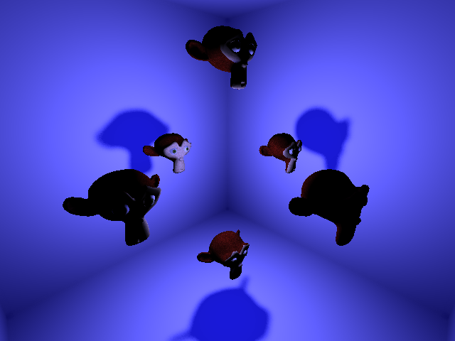
Finally, as mentioned previously, the r2 package allows both optional box blurring and mipmap generation for shadow maps. Both blurring and mipmapping can reduce aliasing artifacts, with the former also allowing the edges of shadows to be significantly softened as a visual effect:

Advantages
The main advantage of variance shadow mapping is that they can essentially be thought of as much better behaved version of basic shadow mapping that just happen to have built-in softening and filtering. Variance shadows typically require far less in the way of scene-specific tuning to get good results.
Disadvantages
One disadvantage of variance shadows is that for large shadow maps, filtering quickly becomes a major bottleneck. On reasonably old hardware such as the Radeon 4670, one 8192x8192 shadow map with two 16-bit components takes too long to filter to give a reliable 60 frames per second rendering rate. Shadow maps of this size are usually used to simulate the influence of the sun over large outdoor scenes.
Types
Variance mapped shadows are represented by the R2ShadowDepthVarianceType type, and can be associated with projective lights.
Rendering of depth-variance images is handled by implementations of the R2ShadowMapRendererType type.